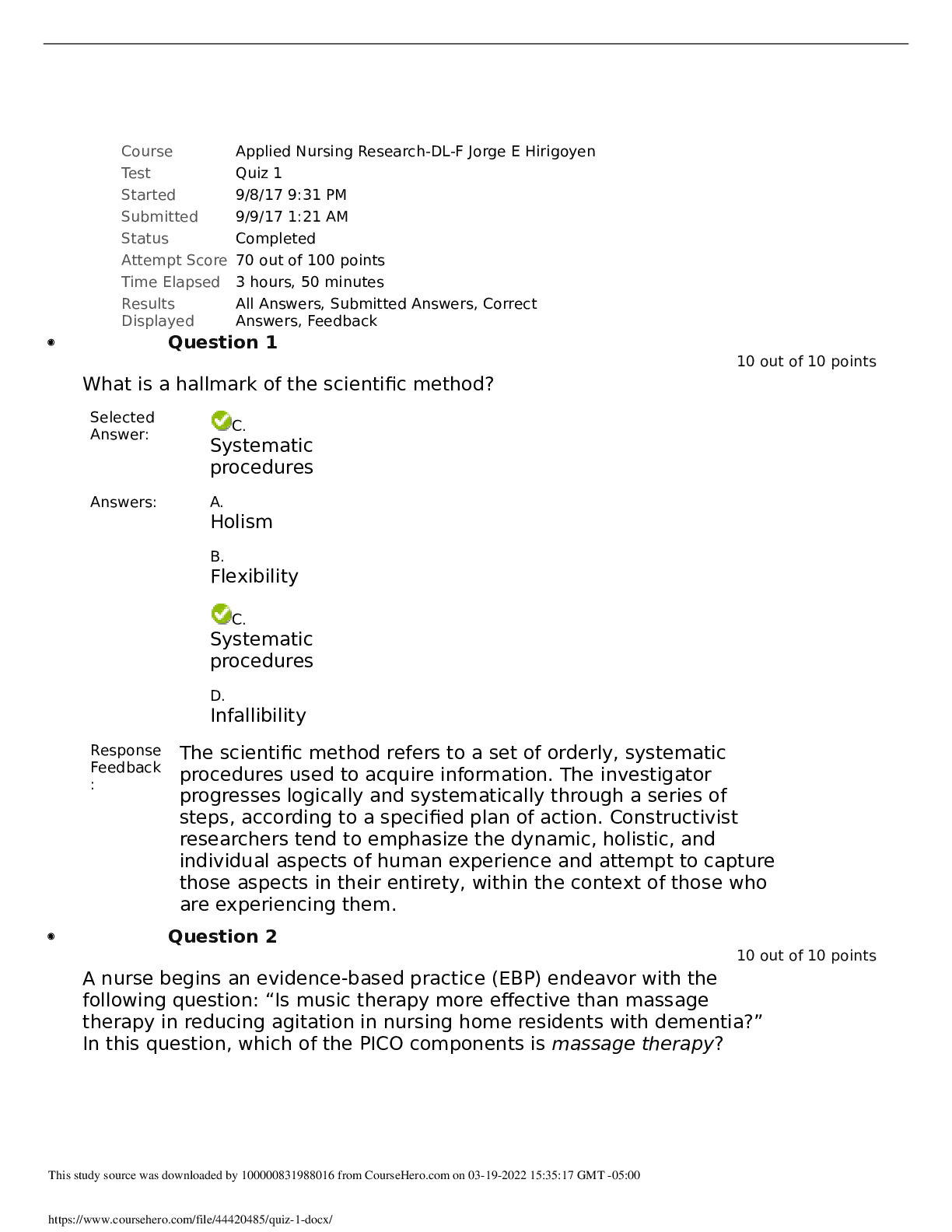
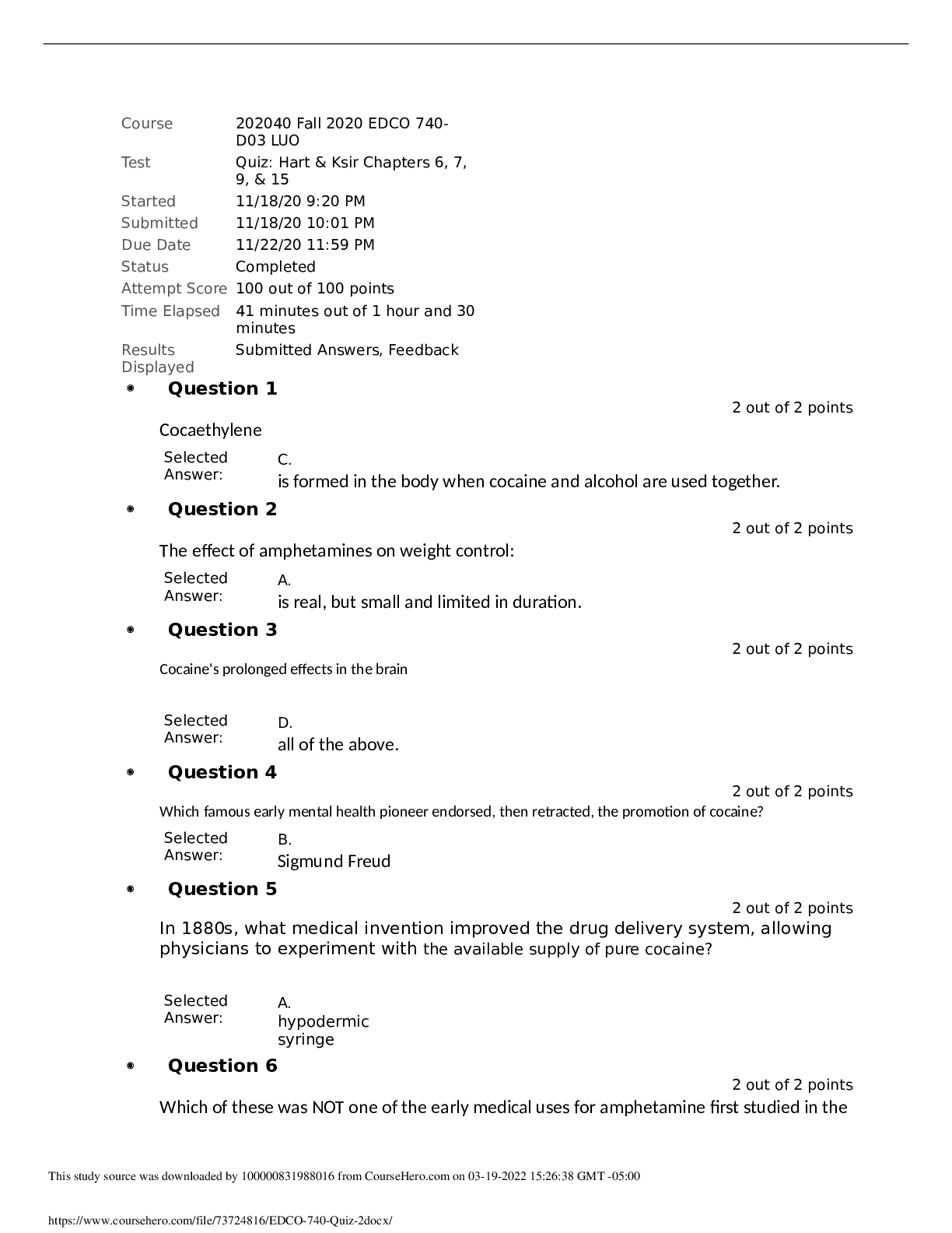
ISYE 6501 Week 6 Homework Latest Update

Document Content and Description Below

Week 6 Homework Question 9.1 Using the same crime data set as in Question 8.2, apply Principal Component Analysis and then create a regression model using the first few principal components. Specif... y your new model in terms of the original variables (not the principal components), and compare its quality to that of your solution to Question 8.2. You can use the R function prcomp for PCA. Note that to first scale the data, you can include scale. = TRUE to scale as part of the PCA function. Don’t forget that, to make a prediction for the new city, you’ll need to unscale the coefficients (i.e., do the scaling calculation in reverse! require("knitr") ## Loading required package: knitr opts_knit$set(root.dir = "~/Desktop/GT OMSA/ISYE 6501/Wk6") Setting up the environment rm(list=ls()) set.seed(1) library(MASS) library(reshape2) library(ggplot2) library(Hmisc) ## Loading required package: lattice ## Loading required package: survival ## Loading required package: Formula ## ## Attaching package: 'Hmisc' ## The following objects are masked from 'package:base': ## ## format.pval, units library(dplyr) ## ## Attaching package: 'dplyr' ## The following objects are masked from 'package:Hmisc': ## ## src, summarize ## The following object is masked from 'package:MASS': ## ## select ## The following objects are masked from 'package:stats': ## ## filter, lag ## The following objects are masked from 'package:base': ## ## intersect, setdiff, setequal, union 1 library(DAAG) ## ## Attaching package: 'DAAG' ## The following object is masked from 'package:survival': ## ## lung ## The following object is masked from 'package:MASS': ## ## hills crime <- read.table("uscrime.txt", header = TRUE) head(crime) ## M So Ed Po1 Po2 LF M.F Pop NW U1 U2 Wealth Ineq ## 1 15.1 1 9.1 5.8 5.6 0.510 95.0 33 30.1 0.108 4.1 3940 26.1 ## 2 14.3 0 11.3 10.3 9.5 0.583 101.2 13 10.2 0.096 3.6 5570 19.4 ## 3 14.2 1 8.9 4.5 4.4 0.533 96.9 18 21.9 0.094 3.3 3180 25.0 ## 4 13.6 0 12.1 14.9 14.1 0.577 99.4 157 8.0 0.102 3.9 6730 16.7 ## 5 14.1 0 12.1 10.9 10.1 0.591 98.5 18 3.0 0.091 2.0 5780 17.4 ## 6 12.1 0 11.0 11.8 11.5 0.547 96.4 25 4.4 0.084 2.9 6890 12.6 ## Prob Time Crime ## 1 0.084602 26.2011 791 ## 2 0.029599 25.2999 1635 ## 3 0.083401 24.3006 578 ## 4 0.015801 29.9012 1969 ## 5 0.041399 21.2998 1234 ## 6 0.034201 20.9995 682 Reading in and viewing the data crime <- read.table("uscrime.txt", header = TRUE) head(crime) ## M So Ed Po1 Po2 LF M.F Pop NW U1 U2 Wealth Ineq ## 1 15.1 1 9.1 5.8 5.6 0.510 95.0 33 30.1 0.108 4.1 3940 26.1 ## 2 14.3 0 11.3 10.3 9.5 0.583 101.2 13 10.2 0.096 3.6 5570 19.4 ## 3 14.2 1 8.9 4.5 4.4 0.533 96.9 18 21.9 0.094 3.3 3180 25.0 ## 4 13.6 0 12.1 14.9 14.1 0.577 99.4 157 8.0 0.102 3.9 6730 16.7 ## 5 14.1 0 12.1 10.9 10.1 0.591 98.5 18 3.0 0.091 2.0 5780 17.4 ## 6 12.1 0 11.0 11.8 11.5 0.547 96.4 25 4.4 0.084 2.9 6890 12.6 ## Prob Time Crime ## 1 0.084602 26.2011 791 ## 2 0.029599 25.2999 1635 ## 3 0.083401 24.3006 578 ## 4 0.015801 29.9012 1969 ## 5 0.041399 21.2998 1234 ## 6 0.034201 20.9995 682 Variable “So” is binary, as this doesnt make sense in a PCA model i am removing it. crime1 <- crime[-2] head(crime1) ## M Ed Po1 Po2 LF M.F Pop NW U1 U2 Wealth Ineq Prob ## 1 15.1 9.1 5.8 5.6 0.510 95.0 33 30.1 0.108 4.1 3940 26.1 0.084602 2 ## 2 14.3 11.3 10.3 9.5 0.583 101.2 13 10.2 0.096 3.6 5570 19.4 0.029599 ## 3 14.2 8.9 4.5 4.4 0.533 96.9 18 21.9 0.094 3.3 3180 25.0 0.083401 ## 4 13.6 12.1 14.9 14.1 0.577 99.4 157 8.0 0.102 3.9 6730 16.7 0.015801 ## 5 14.1 12.1 10.9 10.1 0.591 98.5 18 3.0 0.091 2.0 5780 17.4 0.041399 ## 6 12.1 11.0 11.8 11.5 0.547 96.4 25 4.4 0.084 2.9 6890 12.6 0.034201 ## Time Crime ## 1 26.2011 791 ## 2 25.2999 1635 ## 3 24.3006 578 ## 4 29.9012 1969 ## 5 21.2998 1234 ## 6 20.9995 682 Running the PCA model based on the crime data pca <- prcomp(crime1[,1:15], scale = TRUE) Summarizing and plotting the PCA summary(pca) ## Importance of components: ## PC1 PC2 PC3 PC4 PC5 PC6 PC7 ## Standard deviation 2.3802 1.6756 1.4202 1.16749 1.03667 0.74864 0.5988 ## Proportion of Variance 0.3777 0.1872 0.1345 0.09087 0.07165 0.03736 0.0239 ## Cumulative Proportion 0.3777 0.5649 0.6993 0.79020 0.86185 0.89921 0.9231 ## PC8 PC9 PC10 PC11 PC12 PC13 ## Standard deviation 0.55069 0.48478 0.44375 0.42652 0.32674 0.26644 ## Proportion of Variance 0.02022 0.01567 0.01313 0.01213 0.00712 0.00473 ## Cumulative Proportion 0.94334 0.95900 0.97213 0.98426 0.99138 0.99611 ## PC14 PC15 ## Standard deviation 0.2324 0.06595 ## Proportion of Variance 0.0036 0.00029 ## Cumulative Proportion 0.9997 1.00000 [Show More]

Last updated: 2 years ago

Preview 1 out of 11 pages