Week 1 Homework ISYE 6501

Week 1 Homework ISYE 6501 5/21/2020 Question 2.1 Describe a situation or problem from your job, everyday life, current events, etc., for which a classification model would be appropriate. List some (up to 5) predicto ...

Week 1 Homework ISYE 6501 5/21/2020 Question 2.1 Describe a situation or problem from your job, everyday life, current events, etc., for which a classification model would be appropriate. List some (up to 5) predictors that you might use. https://www.forbes.com/sites/shaharziv/2020/05/14/exclusive-proposal-dont-give-americans-equal-1200-second-stimulus-checks-save-35- billion/#55f2eb9056ec If the US federal government wants to more efficiently distribute stimulus funds, they could vary the amount of money that goes to each household. Residents of states with a higher cost of living would get more money, and residents of states with a lower cost of living would get less money. In addition, families with more children would still get more money. Finally, people who have filed for unemployment would get a larger stimulus than people who are currently employed. In summary, here are the predictors that could be used to determine the amount of stimulus issued by the government: 1. Yearly Income 2. Cost of Living in State of Residence 3. 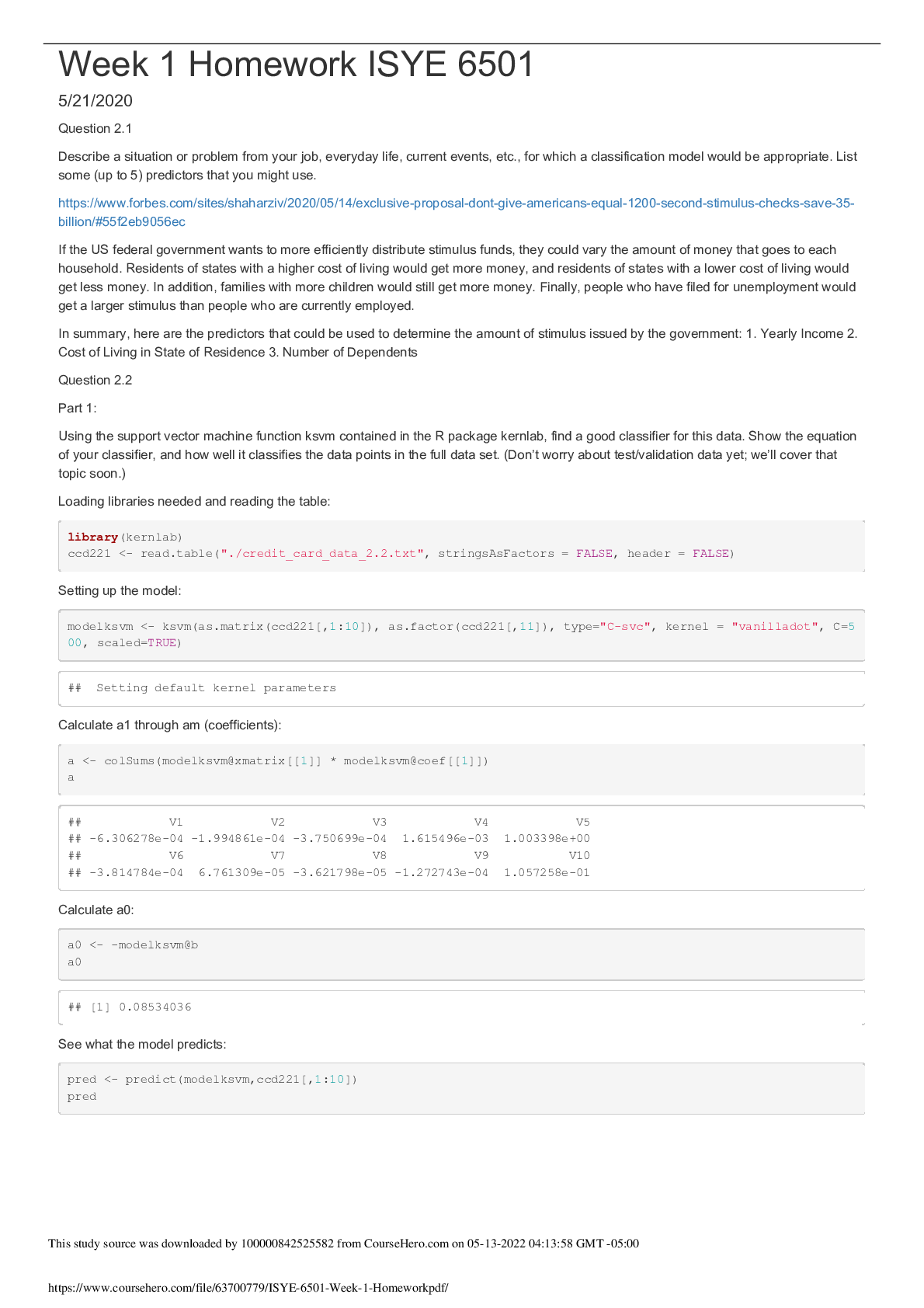Number of Dependents Question 2.2 Part 1: Using the support vector machine function ksvm contained in the R package kernlab, find a good classifier for this data. Show the equation of your classifier, and how well it classifies the data points in the full data set. (Don’t worry about test/validation data yet; we’ll cover that topic soon.) Loading libraries needed and reading the table: library(kernlab) ccd221 <- read.table("./credit_card_data_2.2.txt", stringsAsFactors = FALSE, header = FALSE) Setting up the model: modelksvm <- ksvm(as.matrix(ccd221[,1:10]), as.factor(ccd221[,11]), type="C-svc", kernel = "vanilladot", C=5 00, scaled=TRUE) ## Setting default kernel parameters Calculate a1 through am (coefficients): a <- colSums(modelksvm@xmatrix[[1]] * modelksvm@coef[[1]]) a ## V1 V2 V3 V4 V5 ## -6.306278e-04 -1.994861e-04 -3.750699e-04 1.615496e-03 1.003398e+00 ## V6 V7 V8 V9 V10 ## -3.814784e-04 6.761309e-05 -3.621798e-05 -1.272743e-04 1.057258e-01 Calculate a0: a0 <- -modelksvm@b a0 ## [1] 0.08534036 See what the model predicts: pred <- predict(modelksvm,ccd221[,1:10]) pred This study source was downloaded by 100000842525582 from CourseHero.com on 05-13-2022 04:13:58 GMT -05:00 https://www.coursehero.com/file/63700779/ISYE-6501-Week-1-Homeworkpdf/ ## [1] 1 1 1 1 1 1 1 1 1 1 0 1 1 0 1 1 1 1 1 1 1 1 1 1 1 1 1 1 1 1 1 1 1 1 1 1 1 ## [38] 1 1 1 1 1 1 1 1 1 1 1 0 0 1 1 1 1 1 1 1 1 0 1 1 1 1 1 1 1 1 1 1 1 1 1 1 0 ## [75] 1 1 1 1 1 1 1 1 1 1 1 1 1 1 1 1 1 1 1 1 1 1 1 1 1 1 1 1 1 1 1 1 1 1 1 1 1 ## [112] 1 1 1 1 1 1 1 1 1 1 1 1 1 1 1 1 1 1 1 1 1 1 1 1 1 1 1 1 1 1 1 1 1 1 1 1 1 ## [149] 1 1 1 1 1 1 1 1 1 1 1 1 1 1 1 1 0 1 1 1 1 1 1 1 1 1 1 1 1 1 1 1 1 1 1 1 1 ## [186] 1 1 1 1 1 1 1 1 1 1 1 1 1 1 1 1 1 1 1 1 1 1 1 1 1 1 1 1 1 1 1 1 1 1 1 0 1 ## [223] 1 1 1 1 1 1 1 1 1 1 1 1 1 1 1 1 1 1 1 1 1 1 1 0 0 0 0 0 0 0 0 0 0 0 0 0 1 ## [260] 0 0 0 0 0 0 0 0 1 0 0 0 0 0 0 0 0 0 0 0 0 0 0 0 0 0 0 0 0 0 0 0 0 1 0 0 0 ## [297] 0 0 0 0 0 0 1 0 1 0 0 0 0 0 1 0 0 0 0 0 0 0 0 0 0 0 0 0 0 0 0 0 0 0 0 1 0 ## [334] 0 0 0 0 0 0 0 0 0 0 0 0 0 0 0 0 0 0 0 0 0 0 0 0 0 0 0 0 0 0 0 0 0 0 0 0 0 ## [371] 0 0 0 0 0 0 0 0 0 0 0 0 0 0 0 0 0 0 0 0 0 0 0 0 0 0 0 0 0 0 0 0 0 0 0 0 0 ## [408] 0 0 0 0 0 0 0 0 0 0 0 0 0 0 0 0 0 0 0 0 0 0 0 0 0 0 0 0 0 0 0 0 0 0 0 0 0 ## [445] 0 0 0 0 0 0 0 0 0 0 0 0 0 0 0 0 0 0 0 0 0 1 1 1 1 1 1 1 1 1 1 1 1 1 1 1 1 ## [482] 1 1 1 1 1 1 1 1 1 1 1 1 1 1 1 1 1 1 1 1 1 1 1 1 1 1 1 1 1 1 1 1 1 1 1 1 1 ## [519] 1 1 1 1 1 1 1 1 1 1 1 1 1 1 1 1 1 1 1 1 1 1 1 1 1 1 1 1 1 1 1 1 1 1 1 0 1 ## [556] 1 1 1 1 1 1 1 1 1 0 1 1 1 1 1 1 0 0 1 0 0 0 0 0 0 0 0 0 0 0 0 0 1 0 0 0 0 ## [593] 0 0 0 0 0 0 0 0 0 0 0 0 0 0 0 0 0 0 0 0 0 0 0 0 0 0 1 0 0 0 0 0 0 0 0 0 0 ## [630] 0 0 0 0 0 0 0 0 0 0 0 0 0 0 0 0 0 0 0 0 0 0 0 0 0 ## Levels: 0 1 See what fraction of the model’s predictions match the actual classification: sum(pred == ccd221[,11]) / nrow(ccd221) ## [1] 0.8639144 modelksvm@error ## [1] 0.1360856 Conclusions: A. Since most of the values in the equation of the classifier were close to zero, I will leave them out. The equation of the classifier would approximate to 1.0049x + 0.8639 (scaled) B. Several values of C got the prediction up to 0.86391. Those C values ranged from 0.01 up to about 500. C. This is potentially an example of overfitting, similar to the birth date example in the lecture videos. The reason for that is that we are using the same dataset for the model’s predictions and the actual classification. Question 2.2 Part 2: You are welcome, but not required, to try other (nonlinear) kernels as well; we’re not covering them in this course, but they can sometimes be useful and might provide better predictions than vanilladot. If lambda is left at 100, which is in the range of acceptable values, rbfdot (0.953), polydot (0.865), laplacedot (1.0), besseldot (0.925), anovadot (0.907), and splinedot (0.979) have higher accuracy than vanilladot (0.864). However, tanhdot (0.722) does not. Stringdot throws an error, obviously. Question 2.2 Part 3: Using the k-nearest-neighbors classification function kknn contained in the R kknn package, suggest a good value of k, and show how well it classifies that data points in the full data set. Don’t forget to scale the data (scale=TRUE in kknn). Loading libraries and reading the table: library(kknn) ccd223 <- read.table("./credit_card_data_2.2.txt", stringsAsFactors = FALSE, header = FALSE) Testing multiple k’s: This study source was downloaded by 100000842525582 from CourseHero.com on 05-13-2022 04:13:58 GMT -05:00 https://www.coursehero.com/file/63700779/ISYE-6501-Week-1-Homeworkpdf/ library(kknn) set.seed(1) modelaccuracy <- function(K){ predknn <- array(0,nrow(ccd223)) for (i in 1:nrow(ccd223)) { modelknn <- kknn(V11~V1+V2+V3+V4+V5+V6