Pump Performance
Pump Performance
1. Determine the transducer voltage bias average value from the data file. Include the 95%
CI for this value.
95% CI = 2.82*10-5
2. Test Pump 1. See procedure in lab manual. Complet
...
Pump Performance
Pump Performance
1. Determine the transducer voltage bias average value from the data file. Include the 95%
CI for this value.
95% CI = 2.82*10-5
2. Test Pump 1. See procedure in lab manual. Complete Table 1 below using average voltage
readings from data logger and corresponding pressure differential, pump head, and power draw
for each flow rate.
Table 1: Pump 1 measurement results
Flow Rate
(gpm)
Voltage
Reading P (psi) (lbf ????? ft/lbm) ?̇ ????(W)
15 4.23 6.05 13.98 183
12 4.47 6.80 15.7 180
9 4.95 8.30 19.2 172
6 5.17 8.98 20.8 166
0 5.99 11.5 26.7 139
3. Test Pump 2. See procedure in lab manual. Complete Table 2 below using average voltage
readings from data logger and corresponding pressure differential, pump head, and power draw
for each flow rate.
Table 2: Pump 2 measurement results
Flow Rate
(gpm)
Voltage
Reading P (psi) (lbf ft/lbm ????? ) ?̇ ????(W)
15 4.48 6.828125 15.782504 185
12 4.82 7.890625 18.2383628 180
9 5.29 9.359375 21.6332263 168
6 5.54 10.140625 23.4390048 159
0 6.09 11.859375 27.4117175 120
4. Plot H (ft-lbf/lbm) vs. Q (gpm) curves for the Pump 1 and Pump 2 tests on the same graph along
with the manufacturer’s rated values.
For convenience, the manufacturer’s data are seen in Table 3 below:
Vo = 2.295 +/–
This study source was downloaded by 100000822447745 from CourseHero.com on 07-17-2022 07:17:25 GMT -05:00
https://www.coursehero.com/file/85749085/LAB3WORKSHEETpdf/ME 460 2 Pump Performance
Table 3: Manufacturer's Data for Grundfos pumps
GPM 0 2 4 6 8 10 12 14 16 18 20
Head 29.9 28.7 27.1 25 22.9 20.6 18 15.5 12.8 10.4 7.6
Figure 1 Plot showing Head Loss vs. Flow Rate Curves with error bars
5. Compare and discuss these three pump curves.
As seen in Figure 1 above, all three curves follow the same inverse relationship trend, in that
as flow rate increases, head loss decreases. Pumps 1 and pumps 2 both have relatively similar
curves, with an almost identical slope. The manufacturer’s values however appear to have a
much steeper slope. A reason for this could arise from the fact that the manufacturers’ values
have more data points in its curve, thereby making its curve more precise. If there were more
data points for the pumps 1 and 2 curves, those curves could possibly look more similar to the
manufacturer’s curve.
6. Test Pumps 1 and 2 in Series. See procedure in lab manual. Complete Table 4 below using
average voltage readings from data logger and corresponding pressure differential, pump head,
and power draw for each flow rate.
5 0
10
15
20
25
30
0 4 8 12 16
Head Loss (lbf-ft/lbm)
Flow Rate (GPM)
Pump 1
Pump 2
Manufactuer's Data
This study source was downloaded by 100000822447745 from CourseHero.com on 07-17-2022 07:17:25 GMT -05:00
https://www.coursehero.com/file/85749085/LAB3WORKSHEETpdf/ME 460 3 Pump Performance
Table 4: Series pumps measurement results
Flow Rate
(gpm)
Voltage
Reading P (psi) (lbf ft/lbm ????? ) ?̇ ????(W)
16 4.74 7.64 17.7 373
15 5.09 8.73 20.2 371
12 6.52 13.2 30.5 356
9 7.45 16.1 37.2 341
6 8.25 18.6 43.0 322
0 9.79 23.4 54.1 322
7. Calculate the predicted H (ft-lbf/lbm) vs. Q (gpm) series pump curve using the results for the
individual tests of Pumps 1 and 2. On the same graph, plot this predicted series curve and the
curve from the actual measured results of the Pumps 1 and 2 series test.
Since pumps 1 and 2 are in series, and because pumps in series operate at a constant
flow rate, calculating the predicted head loss values can easily be obtained by adding
the head losses measured at the same flow rates together for pumps 1 and 2. For
example, Htot at 15 GPM can be calculated by adding Hpump1 at 15 GPM and Hpump2 at
15 GPM together.
Figure 2 Plot showing Head Loss vs. Flow Rate Curves for pumps 1 & 2 in series with error bars
0
10
20
30
40
50
60
0 5 10 15 20
Head Loss (lbf-ft/lbm)
Flow Rate (GPM)
Measured Values
Predicted Values
This study source was downloaded by 100000822447745 from CourseHero.com on 07-17-2022 07:17:25 GMT -05:00
https://www.coursehero.com/file/85749085/LAB3WORKSHEETpdf/ME 460 4 Pump Performance
8. Compare and discuss these two curves.
As seen in Figure 2 above, both curves follow the same pattern, in that head loss decreases as
flow rate increases. At 0 GPM, both the predicted and measured head loss values are nearly
equal, and as the flow rate increases, the predicted and measured head loss values slowly
grow a little further apart from each other. Throughout the curve, the predicted head loss
values are calculated to be a little higher than the measure values. The highest gap between
predicted and measured head losses occurs at 15 GPM, where the predicted head loss value is
50% higher than the measured head loss value. A reason for this could be a result of
experimental error from the lab.
9. Test Pumps 1 and 2 in Parallel. See procedure in lab manual. Complete Error! Reference
source not found. below using average voltage readings from data logger and corresponding
pressure differential, pump head, and power draw for each flow rate.
Table 5: Parallel pumps measurement results
Flow Rate
(gpm)
Voltage
Reading P (psi) (lbf ft/lbm ????? ) ?̇ ????(W)
20 4.93 8.234375 19.0329053 346
15 5.25 9.234375 21.3443018 328
10 5.56 10.203125 23.5834671 309
5 5.75 10.796875 24.9558587 291
0 5.99 11.546875 26.6894061 267
*Replace with full open flow rate and delete this footnote
10. Calculate the predicted H (ft-lbf/lbm) vs. Q (gpm) parallel pump curve using the results for the
individual tests of Pumps 1 and 2. On the same graph, plot this predicted parallel curve and the
curve from the actual measured results of the Pumps 1 and 2 parallel tests.
Since pumps 1 and 2 are in parallel, and because pumps in series operate at a constant
head, calculating the predicted flow rate values have to be obtained with the quadratic
formula. Polynomial curves for pumps 1 and 2 were obtained by plotting the pumps 1
and 2 data, and then using its polynomial trendline equation. Using that equation for
each individual measured head loss values for pumps 1 and 2, the flow rate is
calculated by using the quadratic formula. Once the flow rates are calculated, those
two parallel flow rate values at pumps 1 and 2 are added together.
[Show More]