Calculus > SOLUTIONS MANUAL > Florida Atlantic University - EEE 5425solutions (All)
Florida Atlantic University - EEE 5425solutions
Document Content and Description Below
Last updated: 3 years ago
Preview 1 out of 82 pages
Instant download
Buy this Document to get the Full Access Instantly
Provided by Students Who Aced it
We Verify Document Content to Gurantee Accuracy
Reviews( 0 )
Document information
Connected school, study & course
About the document
Uploaded On
Apr 17, 2021
Number of pages
82
Written in
All

Additional information
This document has been written for:
Uploaded
Apr 17, 2021
Downloads
0
Views
130
Document Keyword Tags
Recommended For You
Get more on SOLUTIONS MANUAL »
Solutions Manual for Thomas' Calculus Early Transcendentals, 1...
Calculus Single and Multivariable. 7e Hughes Hallett, McCallum...
.png)
Calculus Early Transcendentals 11e Howard Anton, Irl Bivens, S...
Solutions Manual For Vector Calculus, 5th Edition by Susan Col...
Solution Manual for Calculus Single Variable 7th Edition by Wi...
Solutions Manual For Calculus 5th Edition by James Stewart, Ko...
Solutions Manual with Test Bank for Thomas' Calculus Early...


Test Bank for Calculus, 2nd Canadian Edition By Michael Calter...
TEST BANK FOR DEBORAH GRAY MORRIS CALCULATE WITH CONFIDENCE 7T...
Test Bank for Thomas' Calculus Early Transcendentals 15th Edit...

Practice Final Exam Solutions - Accelerated Multivariable Calc...

Broward College - MAC 2311Calculus Exam 1 ( all solutions are...

Math Calculus ESSON The Equation of the Tangent line 5.2 Act...
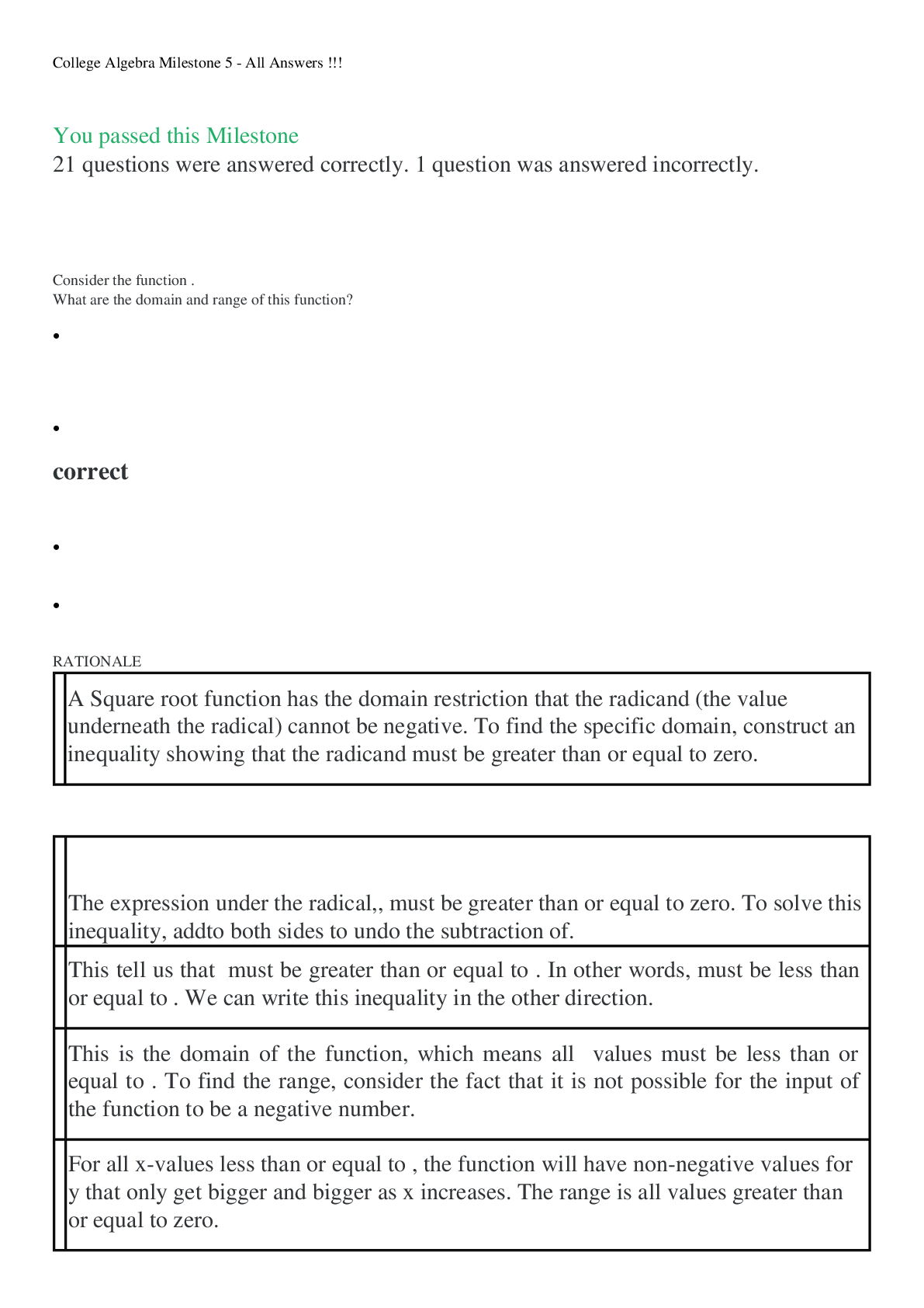
College Algebra Milestone 5 - All Answers !!! | 22 Questions,...

AP® Calculus BC Exams 2012 - 2017 ( all with answer keys ) DOW...
Calculus Early Transcendentals Single Variable 4th Edition By...
Instructors Manual for Precalculus 6th edition by Daniel S. Mi...

