Statistics > QUESTIONS & ANSWERS > TEST BANK FOR STAT C100. COMPLETE GUIDE FOR FINAL EXAM PREPARATION. GRADED A. (All)
TEST BANK FOR STAT C100. COMPLETE GUIDE FOR FINAL EXAM PREPARATION. GRADED A.
Document Content and Description Below
Last updated: 3 years ago
Preview 1 out of 30 pages
Instant download

Buy this Document to get the Full Access Instantly
Provided by Students Who Aced it
We Verify Document Content to Gurantee Accuracy
Reviews( 0 )
Document information
Connected school, study & course
About the document
Uploaded On
May 01, 2021
Number of pages
30
Written in
All

Additional information
This document has been written for:
Uploaded
May 01, 2021
Downloads
0
Views
143
Document Keyword Tags
Recommended For You
Get more on QUESTIONS & ANSWERS ».png)
C100 WGU Objective Assessment Questions and Answers Already Pa...
.png)

Hepatitis C 100 Questions & Answers A Lahey Clinic Guide-Jones...
.png)
WGU C100 Introduction To Humanities Questions and Answers Grad...

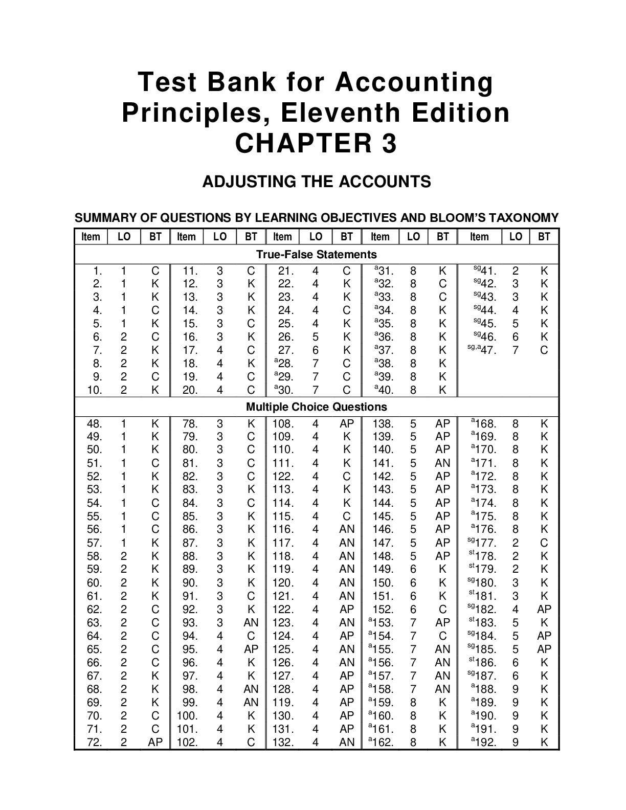
Test Bank for Accounting Principles, Eleventh Edition. ACC100....

C100 WGU Objective Assessment Questions and Answers, Graded A
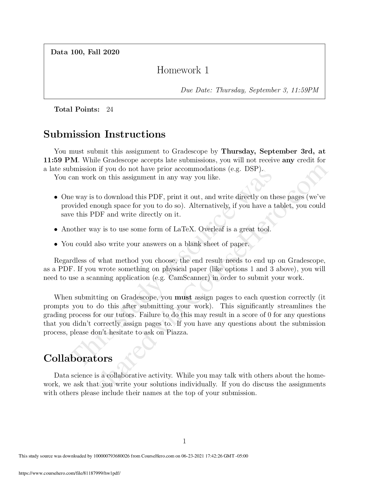
University of California, BerkeleyCS C100hw1 FALL 2020 < VERIF...

Test bank- Essentials-of-Understanding-Psychology-11th-Edition...
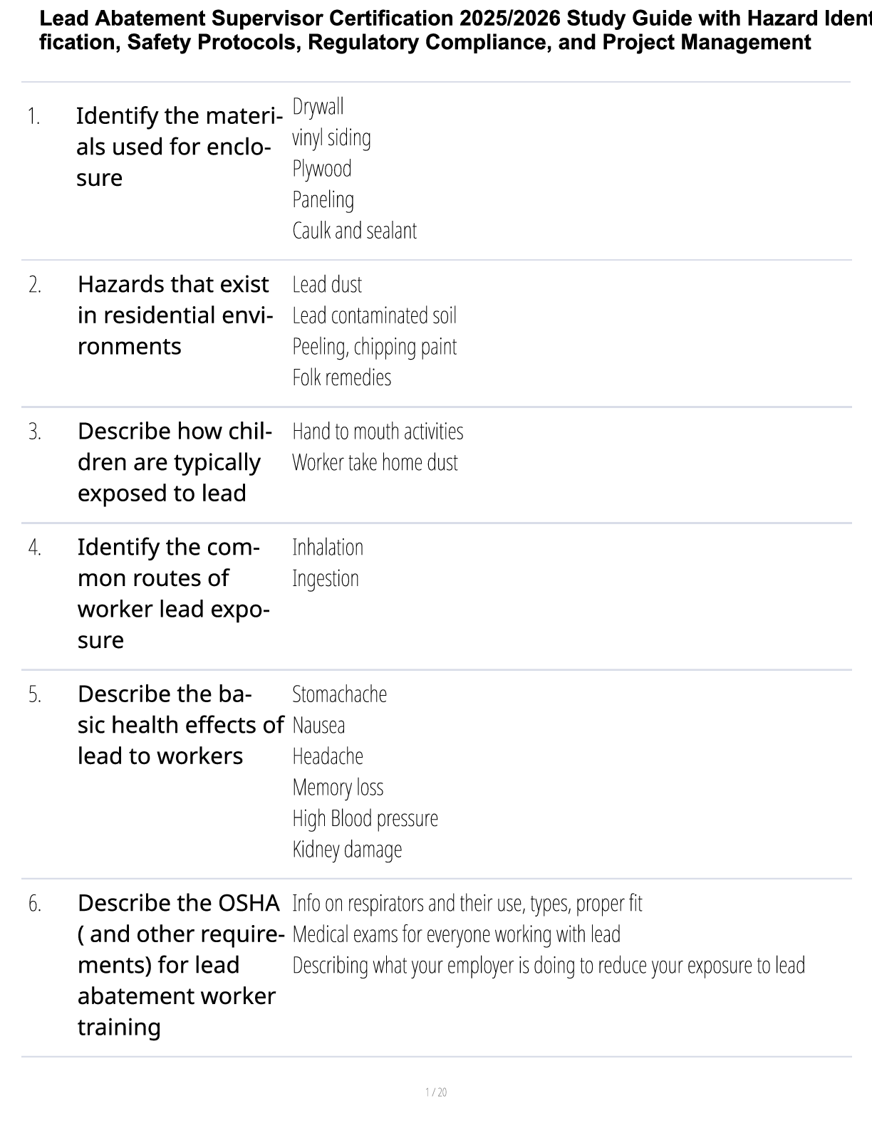
WGU C100 Humanities 2025/2026 Study Guide with Cultural Histor...

Broward College - BSC1005L 1101IB_1201_L05_Enzymes BC custom
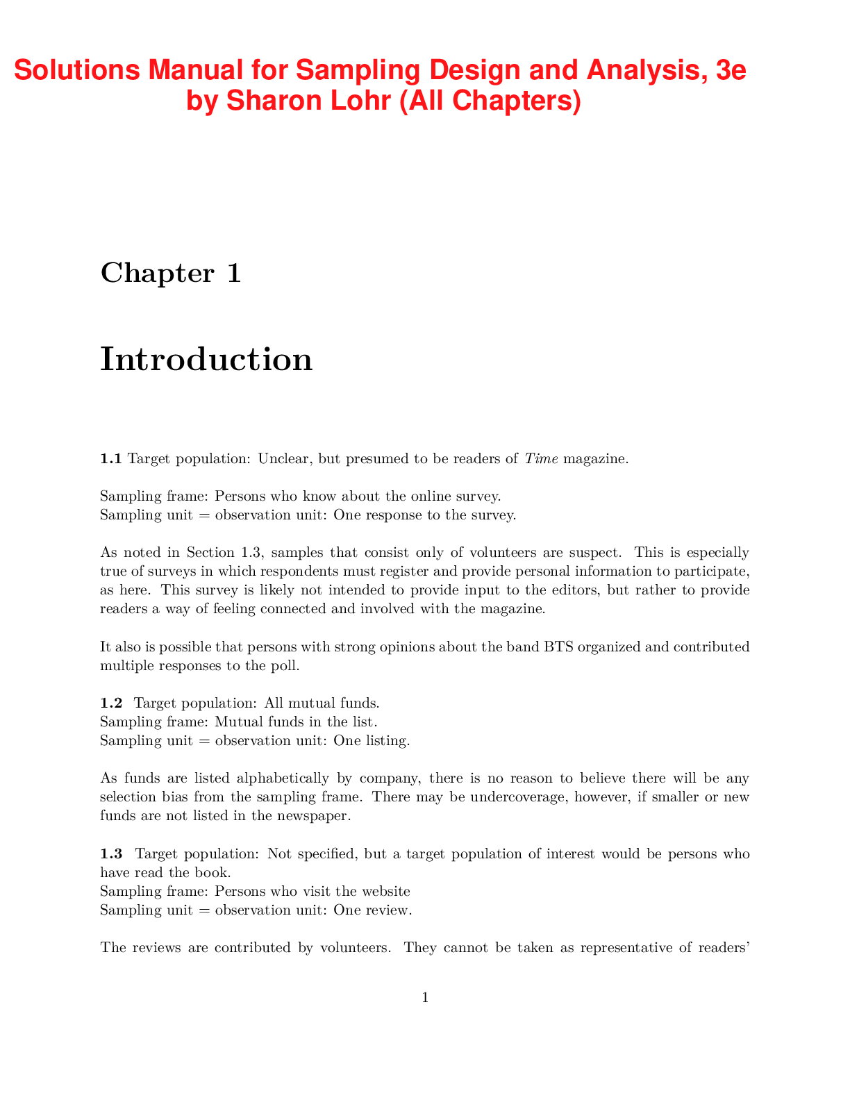
Sampling Design and Analysis, 3e by Sharon Lohr (Solutions Man...
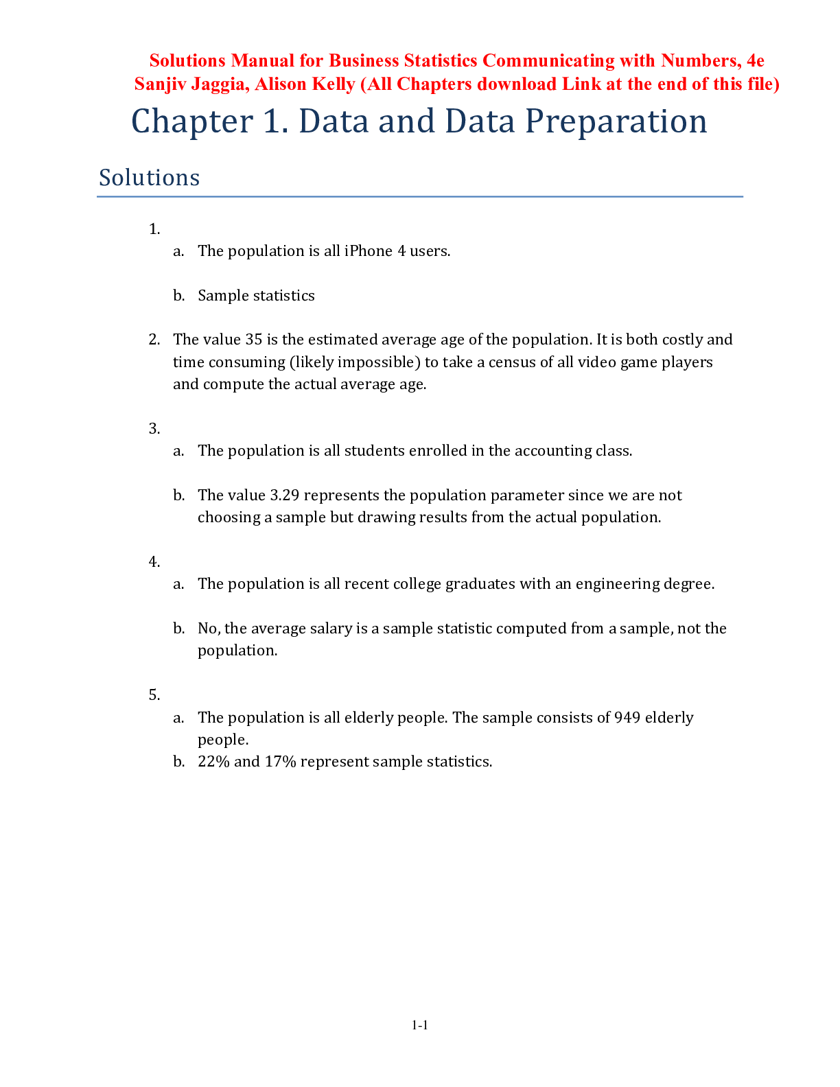
Solutions Manual for Business Statistics Communicating with Nu...
.png)
Introduction to Statistical Investigations, 2e Tintle, Chance,...
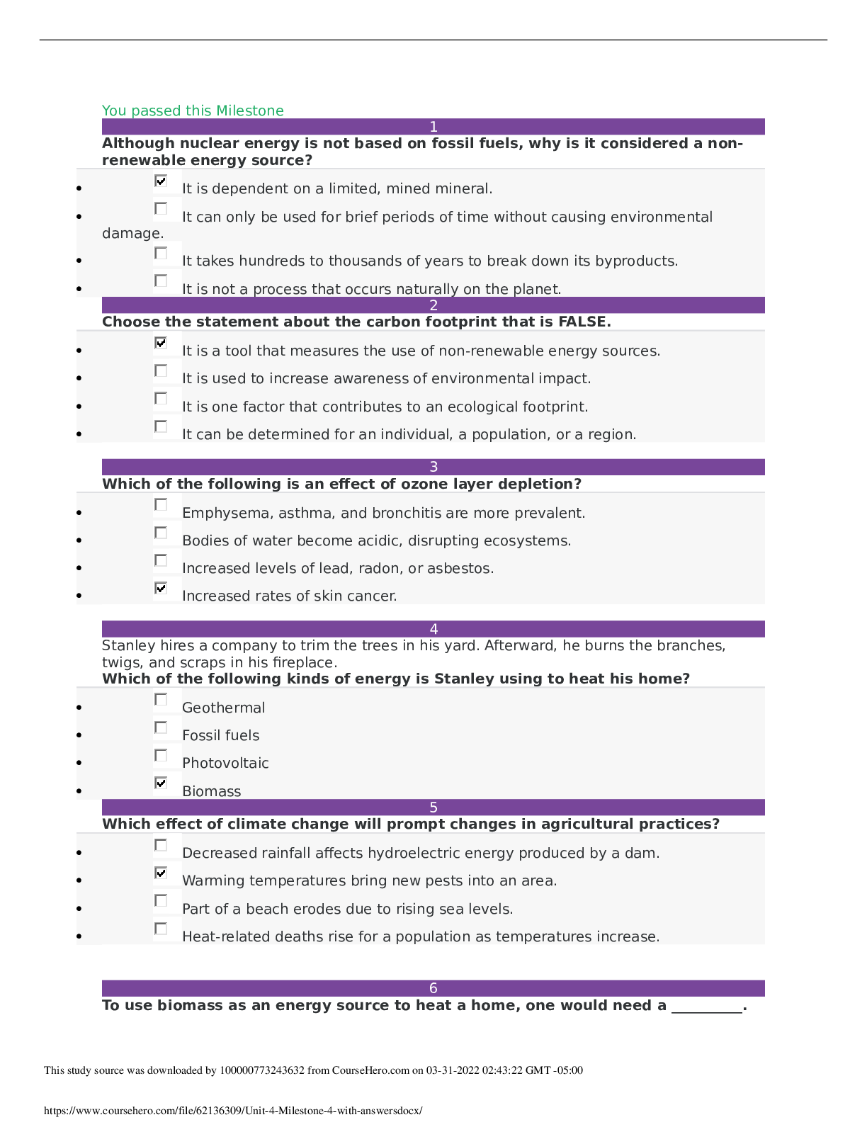
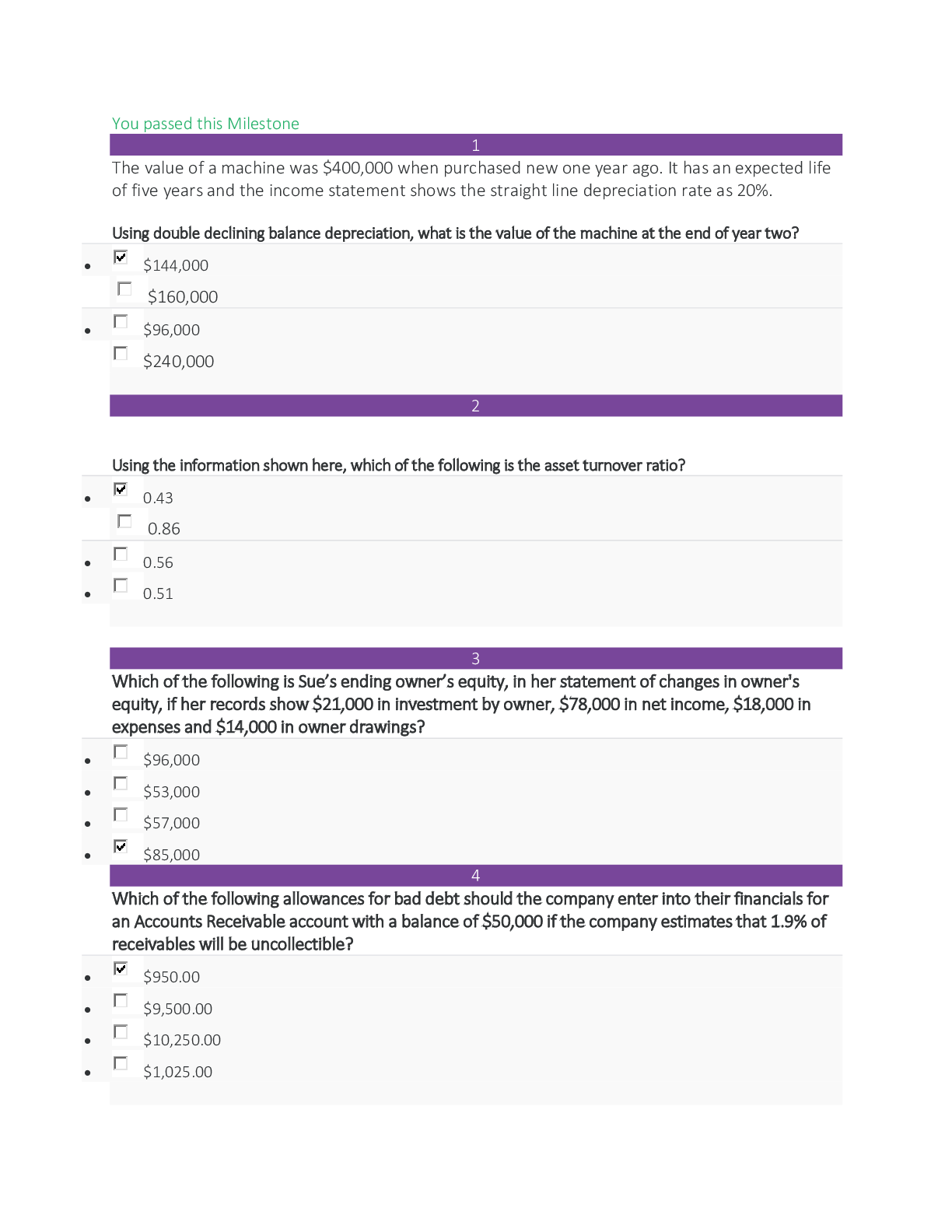
ACC 100_Unit 4 Milestone 4. SOPHIA ACCOUNTING Unit 4 Milestone...


.png)

.png)

