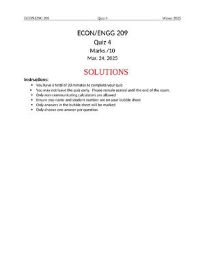
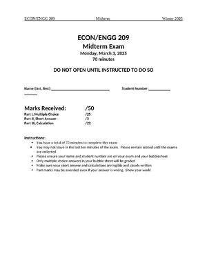
Economics > EXAM > ECONOMICS MISC Markets, Demand and Supply - Linear Demand and Supply functions PRACTICE ACTIVITIES (All)
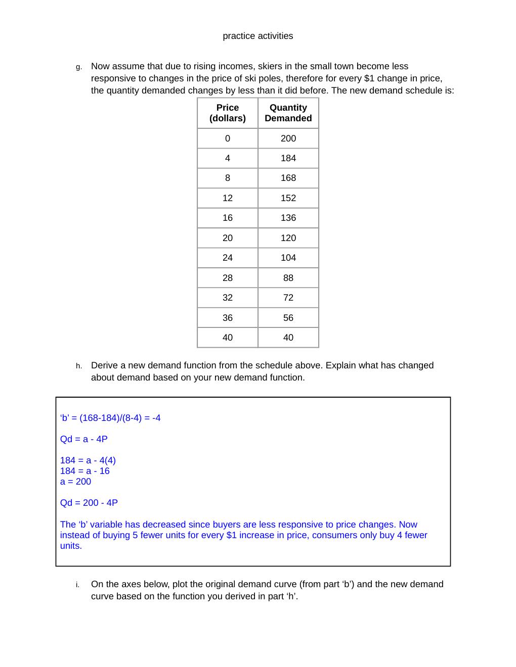
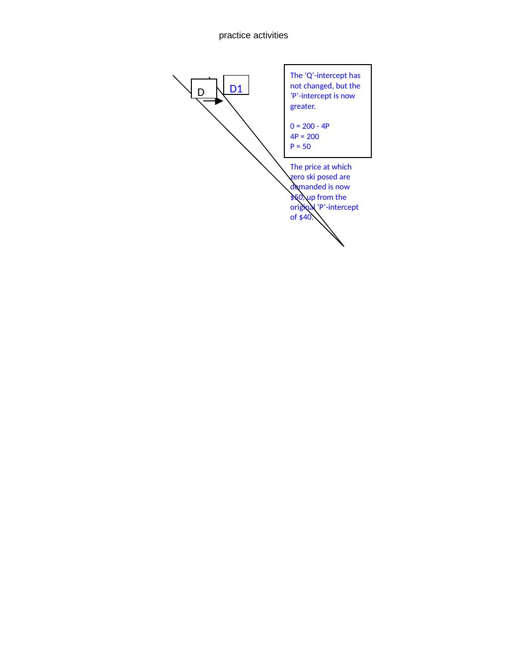
ECONOMICS MISC Markets, Demand and Supply - Linear Demand and Supply functions PRACTICE ACTIVITIES
Document Content and Description Below
Last updated: 4 hours ago
Preview 5 out of 20 pages
Instant download
Buy this Document to get the Full Access Instantly
Provided by Students Who Aced it
We Verify Document Content to Gurantee Accuracy
Reviews( 0 )
Document information
Connected school, study & course
About the document
Uploaded On
Nov 21, 2026
Number of pages
20
Written in
All

Additional information
This document has been written for:
Uploaded
Nov 21, 2026
Downloads
0
Views
10
Topic Tags
Recommended For You
Get more on EXAM »
Test Bank for The Economics of Money, Banking and Financial Ma...
Test Bank For Matching Supply with Demand An Introduction to O...
Solution Manual For Matching Supply with Demand An Introductio...
SOLUTIONS MANUAL for Labor Economics 9th Edition by George Bor...

Solution Manual For Economics, 11th Edition by John Sloman Dea...

Solutions Manual for Economics, 11th Edition by John Sloman De...
Test Bank For Byrd & Chen's Canadian Tax Principles (vol 2) 20...
eBook Economics 11th Edition By John Sloman, Dean Garratt, Jon...

Economics, 11th Edition by John Sloman Dean Garratt Jon Guest...
AQA A Level Economics Paper 2 | ECON 3140 National and Interna...