Electrical Engineering > Lab Experiment > University of Alberta MECE 390 Lab 2 (All)
University of Alberta MECE 390 Lab 2
Document Content and Description Below
Last updated: 3 years ago
Preview 1 out of 2 pages
Instant download
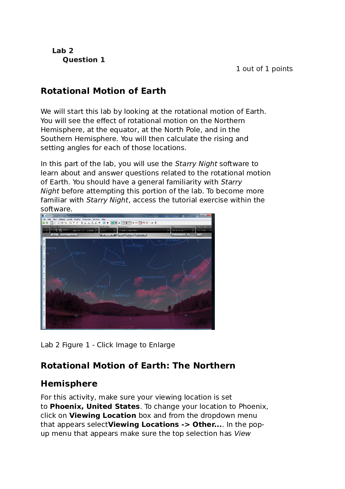
Buy this Document to get the Full Access Instantly
Provided by Students Who Aced it
We Verify Document Content to Gurantee Accuracy
Reviews( 0 )
Document information
Connected school, study & course
About the document
Uploaded On
May 27, 2021
Number of pages
2
Written in
All

Additional information
This document has been written for:
Uploaded
May 27, 2021
Downloads
0
Views
139
Topic Tags
Recommended For You
Get more on Lab Experiment »
Introduction to Electric Circuits 9th Edition By James Svobod...

Illustrated Guide to the National Electrical Code, 7e Charles...
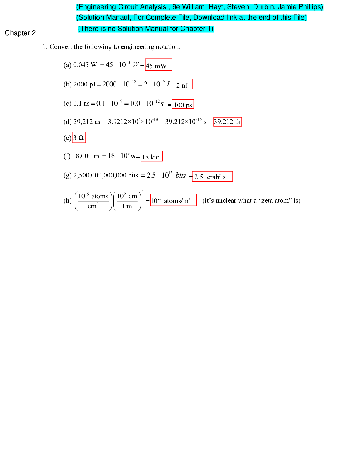
Engineering Circuit Analysis , 9e William Hayt, Steven Durbi...
Energy-Efficient Electrical Systems for Buildings, 1e Moncef K...
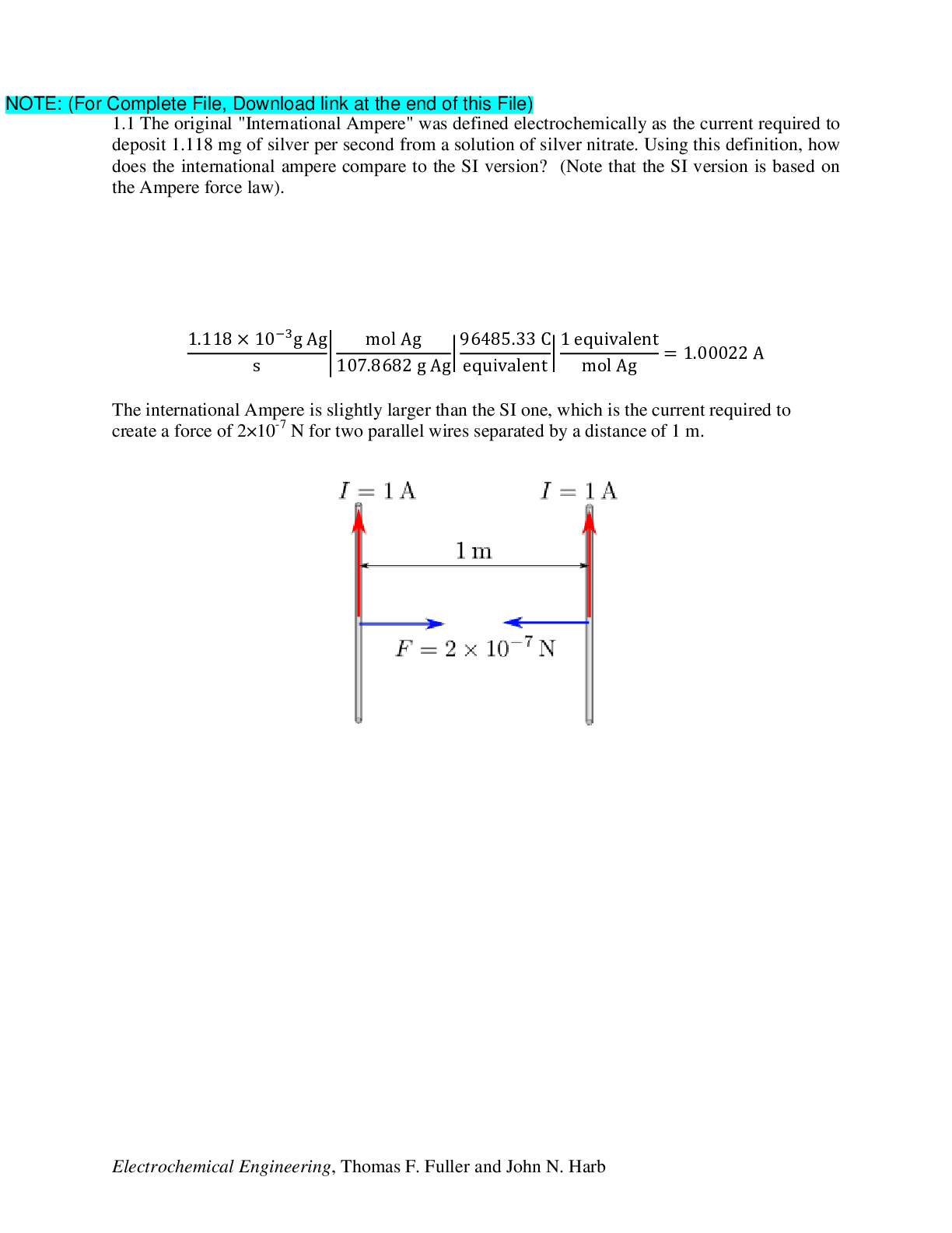
Electrochemical Engineering, 1e Thomas Fuller (Solution Manual...

Electrical Engineering Concepts and Applications 1e Reza Zekav...

Electric Circuits, 11th Edition by James Nilsson, Susan Riedel...
Dopants and Defects in Semiconductors, 2e Matthew McCluskey, E...
Delmar's Standard Textbook of Electricity, 6e Stephen Herman (...
Delmar's Standard Textbook of Electricity, 6e Stephen Herman (...

Single-Inductor Multiple-Output Converters Topologies, Impleme...

An Introduction to Electrical Science, 1e Adrian Waygood (Test...

Advanced Electromagnetic Wave Propagation Methods, 1e by Guill...
Electricity for Refrigeration, Heating, and Air Conditioning,...
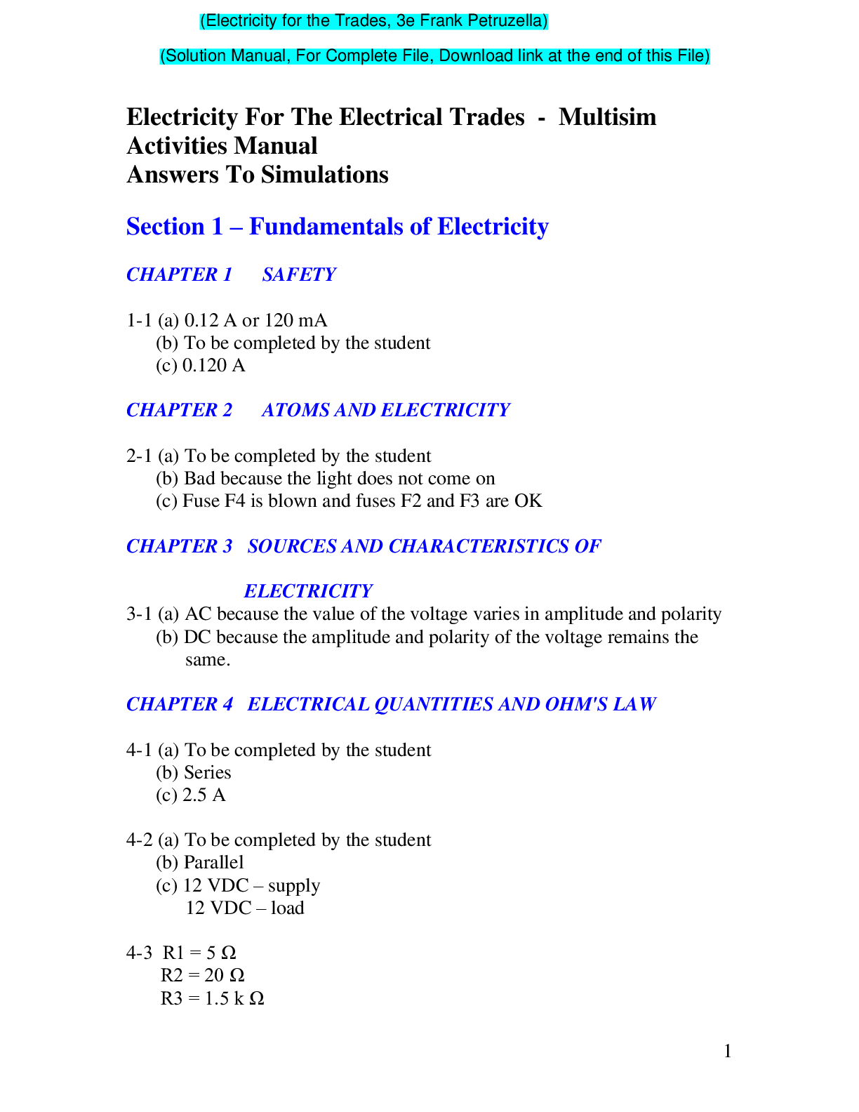
Electricity for the Trades, 3e Frank Petruzella (Solution Manu...


Electricity for Refrigeration, Heating, and Air Conditioning,...
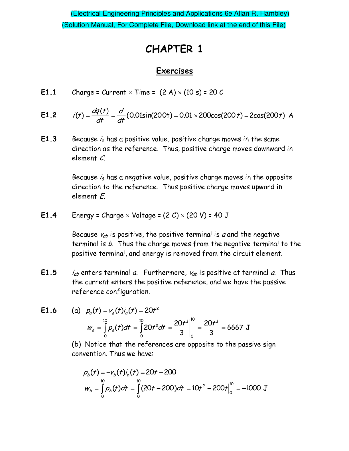
Electrical Engineering Principles and Applications 6e Allan R....