12/7/2019 Week 12 Homework: Simulation - ISYE-6644-OAN
https://gatech.instructure.com/courses/75320/quizzes/69213 1/13
Week 12 Homework
Due Nov 17 at 11:59pm Points 17 Questions 17
Available after Nov 8 at 8am Time L
...
12/7/2019 Week 12 Homework: Simulation - ISYE-6644-OAN
https://gatech.instructure.com/courses/75320/quizzes/69213 1/13
Week 12 Homework
Due Nov 17 at 11:59pm Points 17 Questions 17
Available after Nov 8 at 8am Time Limit None
Attempt History
Attempt Time Score
LATEST Attempt 1 1,965 minutes 13 out of 17
Score for this quiz: 13 out of 17
Submitted Nov 17 at 8:18pm
This attempt took 1,965 minutes.
Question 1 0 / 1 pts
(Lesson 8.1: Introduction to Input Modeling.) It's GIGO time! Let's consider
an queueing system with Exp( ) interarrivals and Exp( ) FIFO
services at a single server. You may recall from some class (either this one
or stochastic processes) that the steady-state expected cycle time (i.e., the
time that the customer is in the system, including wait + service) is
.
If you were to try this out in Arena, let's say with
interarrivals and services (note the notation change
between my usual "Exp" and Arena's ), then we'd get
. Go ahead, see for yourself in Arena, but make
sure that you run the system for 100,000 or so customers so that you can be
sure that you're in steady-state!
Finally, here's the GIGO question, which will show what can happen when
you mis-model a component of your process: What is the (approximate)
steady-state expected cycle time if you have i.i.d. interarrivals
instead of interarrivals? Note that both interarrival
distributions have the same mean (10), but that doesn't necessarily imply
that they'll have the same expected cycle times. Hint: You may want to use
Arena as described above.12/7/2019 Week 12 Homework: Simulation - ISYE-6644-OAN
https://gatech.instructure.com/courses/75320/quizzes/69213 2/13
a. about 1
Y You Answered ou Answered b. about 10
orrect Answer orrect Answer c. about 23
d. about 40
e. about 62
(c). The case has waaaay smaller tails than the , so it's
reasonable to assume that the cycle times will tend to be lower for the
case. In fact, after 100,000 customers in Arena, I got an
average time of 23.5. Thus, (c) is the right answer.
Question 2 1 / 1 pts
(Lesson 8.2: Identifying Distributions.) Let's play Name That Distribution!
The number of times a "3" comes up in 10 dice tosses.
a. Bernoulli
Correct! Correct! b. Binomial
c. Geometric
d. Negative Binomial
e. Pareto
(b).12/7/2019 Week 12 Homework: Simulation - ISYE-6644-OAN
https://gatech.instructure.com/courses/75320/quizzes/69213 3/13
Question 3 1 / 1 pts
(Lesson 8.2: Identifying Distributions.) Name That Distribution!
The number of dice tosses until a 3 comes up.
a. Bernoulli
b. Binomial
Correct! Correct! c. Geometric
d. Negative Binomial
e. Pareto
(c).
Question 4 0 / 1 pts
(Lesson 8.2: Identifying Distributions.) Name That Distribution!
The number of dice tosses until a 3 comes up for the 4th time.
a. Bernoulli
b. Binomial
Y You Answered ou Answered c. Geometric
orrect Answer orrect Answer d. Negative Binomial
e. Pareto12/7/2019 Week 12 Homework: Simulation - ISYE-6644-OAN
https://gatech.instructure.com/courses/75320/quizzes/69213 4/13
(d).
Question 5 1 / 1 pts
(Lesson 8.2: Identifying Distributions.) Name That Distribution!
IQs
a. Uniform
Correct! Correct! b. Normal
c. Exponential
d. Weibull
e. Pareto
(b).
Question 6 1 / 1 pts
(Lesson 8.2: Identifying Distributions.) Name That Distribution!
Cases in which you have limited information, e.g., you only know the min,
max, and "most likely" values that a random variable can take.
a. Bernoulli
b. Poisson12/7/2019 Week 12 Homework: Simulation - ISYE-6644-OAN
https://gatech.instructure.com/courses/75320/quizzes/69213 5/13
Correct! Correct! c. Triangular
d. Weibull
e. Pareto
(c).
Question 7 1 / 1 pts
(Lesson 8.3: Unbiased Point Estimation.) Find the sample variance of
a. 0
b. 1
c. 4
Correct! Correct! d. 14/3
e. 6
So the answer is (d).
Question 8 0 / 1 pts12/7/2019 Week 12 Homework: Simulation - ISYE-6644-OAN
https://gatech.instructure.com/courses/75320/quizzes/69213 6/13
(Lesson 8.3: Unbiased Point Estimation.) If are i.i.d. Pois(6),
what is the expected value of the sample variance ?
a. 1/6
Y You Answered ou Answered b. 1/36
orrect Answer orrect Answer c. 6
d. 36
e. 60
is always unbiased for the variance of . Thus, we have
. So the answer is (c).
Question 9 1 / 1 pts
(Lesson 8.4: Mean Squared Error.) Suppose that estimator A has bias = 3
and variance = 12, while estimator B has bias -2 and variance = 14. Which
estimator (A or B) has the lower mean squared error?
a. A
Correct! Correct! b. B
MSE = Bias + Var, so
Thus, B has lower MSE.12/7/2019 Week 12 Homework: Simulation - ISYE-6644-OAN
https://gatech.instructure.com/courses/75320/quizzes/69213 7/13
Question 10 1 / 1 pts
(Lessons 8.5 and 8.6: Maximum Likelihood Estimators.) If ,
, and are i.i.d. realizations from a Nor( ) distribution,
what is the value of the maximum likelihood estimate for the variance ?
a. 0
b. 1
Correct! Correct! c. 8/3
d. 4
e. None of the above
We know from a class example that
Thus, the answer is (c).
Question 11 1 / 1 pts
(Lessons 8.5 and 8.6: Maximum Likelihood Estimators.) Suppose we
observe the Pois realizations and . What is the
maximum likelihood estimate of ?
a. 0
Correct! Correct! b. 5
c. 2512/7/2019 Week 12 Homework: Simulation - ISYE-6644-OAN
https://gatech.instructure.com/courses/75320/quizzes/69213 8/13
d. 1/5
e. 1/25
I don't remember if we derived the MLE of in class or not, but here's
how anyway. The likelihood function is
Thus,
This implies that
Setting the derivative to 0 and solving yields . Duh! What
a surprise! So the answer is (b).
Question 12 1 / 1 pts
(Lesson 8.7: Invariance Property of MLEs) Suppose that we have a number
of observations from a Pois distribution, and it turns out that the MLE for
is . What's the maximum likelihood estimate of ?
Correct! Correct! a. 0.1404
b. 5
c. 2512/7/2019 Week 12 Homework: Simulation - ISYE-6644-OAN
https://gatech.instructure.com/courses/75320/quizzes/69213 9/13
d. 1/5
e. 1/25
By invariance,
so that we have
Thus, the answer is (a).
Question 13 1 / 1 pts
(Lesson 8.8: Method of Moments.) BONUS: Suppose that we observe , ,
and . What's the method of moments estimate of ?
a. 5
b. 25
Correct! Correct! c. 35.7
d. 1/5
e. 1/25
The MOM estimator for is . Thus, the answer is (c).12/7/2019 Week 12 Homework: Simulation - ISYE-6644-OAN
https://gatech.instructure.com/courses/75320/quizzes/69213 10/13
Question 14 1 / 1 pts
(Lesson 8.9: Goodness-of-Fit Tests.) Suppose we're conducting a
goodness-of-fit test with Type I error rate to determine whether or not 100
i.i.d. observations are from a lognormal distribution with unknown parameters
. If we divide the observations into 5 equal-probability intervals and we
observe a g-o-f statistic of , will we ACCEPT (i.e., fail to reject) or REJECT
the null hypothesis of lognormality?
Accept
Correct! Correct! Reject
Note that the test has degrees of freedom. Then
so we REJECT even though we're being conservative with such a
small !
Question 15 1 / 1 pts
(Lessons 8.10 and 8.11: Goodness-of-Fit Test.) This problem has a really
long description, but the question itself will be very short! Be patient!
The number of defects in printed circuit boards is hypothesized to follow a
Geometric() distribution. A random sample of printed boards has been
collected, and the number of defects observed. Here are the results.
Number of Defects Observed Frequency
1 34
2 18
3 2
4 912/7/2019 Week 12 Homework: Simulation - ISYE-6644-OAN
https://gatech.instructure.com/courses/75320/quizzes/69213 11/13
5 7
It turns out that the MLE of for the Geom() is . (See the following proof if you
don't believe me!)
Proof: The likelihood function is
Thus,
and so,
Solving for gives the MLE .
So in this particular case, we have:
and thus
Anyhow, we are interested in performing a goodness-of-fit test to test the
Geometric hypothesis. To this end, let's get the test statistic, ? To do so, let's
make a little table, assuming that is correct. Note that the expected number
of observations having a certain value is . Also note that I've combined the
entries in the last row () so the probabilities add up to one.
1 0.4762 33.33 34
2 0.2494 17.46 18
3 0.1307 9.15 2
4 0.0684 4.79 9
0.0752 5.27 7
1.0000 70 70
Technically speaking, we really ought to combine the last two cells, since .
Let's do so to get the following new-and-improved table.
1 0.4762 33.33 34
2 0.2494 17.46 1812/7/2019 Week 12 Homework: Simulation - ISYE-6644-OAN
https://gatech.instructure.com/courses/75320/quizzes/69213 12/13
3 0.1307 9.15 2
0.1436 10.06 16
1.0000 70 70
Thus, the test statistic is
Now, let's use our old friend in our test. Let denote the number of cells (that
we ultimately ended up with) and let denote the number of parameters we
had to estimate. Then we compare against . So after all this time, here's my
question: Do we ACCEPT (i.e., fail to reject) or REJECT the Geometric
hypothesis?
a. Accept
Correct! Correct! b. Reject
Since , we REJECT. That wasn't so bad, was it?
Question 16 0 / 1 pts
(Lesson 8.12: Kolmogorov--Smirnov Test.) Consider the PRN's . Use
Kolmogorov-Smirnov with to test to see if these numbers are indeed
uniform. Do we ACCEPT (i.e., fail to reject) or REJECT uniformity?
orrect Answer orrect Answer a. Accept
Y You Answered ou Answered b. Reject12/7/2019 Week 12 Homework: Simulation - ISYE-6644-OAN
https://gatech.instructure.com/courses/75320/quizzes/69213 13/13
Need to make a little table, where the denote the ordered PRN's.
1 2 3
0.1 0.2 0.9
0.233 0.467 0.1
0.1 - 0.233
Thus, , and , and so
finally the K-S test stat is .
The necessary quantile is .
Since , we ACCEPT (i.e., fail to reject) uniformity (though it's kind of a
joke since it's only based on 3 observations)
Question 17 1 / 1 pts
(Lesson 8.14: Arena Input Analyzer.) You don't have to turn anything in for
this, but I'd simply like you to play around with the Arena Input Analyzer. So,
did you look at the Input Analyzer? (You should answer YES.)
Correct! Correct! a. Yes
b. No
Quiz Score: 13 out of 17
[Show More]















 Charles Herrick - 100 Q&A About Alcoholism & Drug Addiction-Jones and Bartlett Publishers, Inc.png)