MATH 533 Week 8 Final Exam Set 3 (100% CORRECT Solution) | Already graded A+

Document Content and Description Below

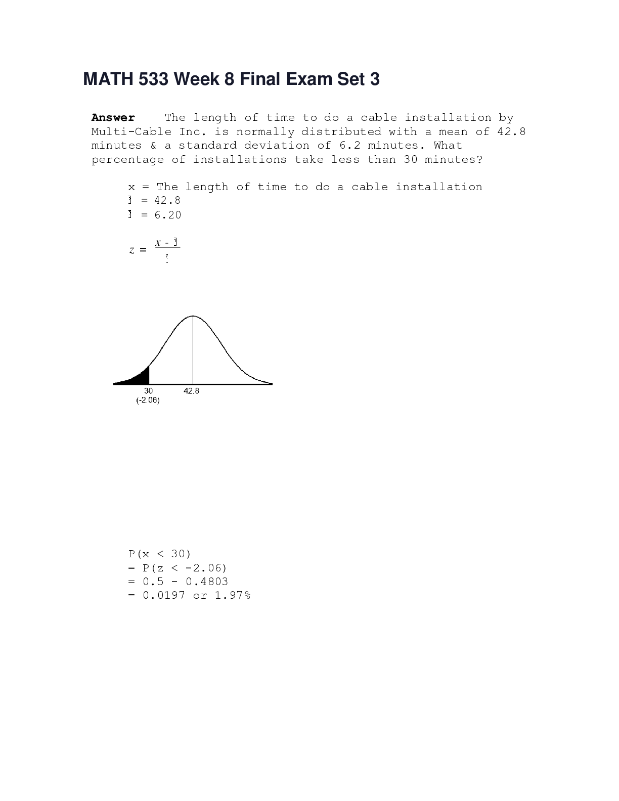
MATH 533 Week 8 Final Exam Set 3 Answer The length of time to do a cable installation by Multi-Cable Inc. is normally distributed with a mean of 42.8 minutes & a standard deviation of 6.2 minutes. ... What percentage of installations take less than 30 minutes? x = The length of time to do a cable installation  = 42.8  = 6.20 z = x -   P(x < 30) = P(z < -2.06) = 0.5 - 0.4803 = 0.0197 or 1.97% Answer Accident claims are checked for completeness by branch offices of Fortune Insurance before they are sent to a regional office for payment. Historically 80% of the claims are complete when they reach the regional office. You select a random sample of 20 claims that have arrived at the regional office. Find the probability that: X = Number of completed forms in sample n = 20 p = 0.80 a. At least 16 claims are complete, P(X  16) = P(X = 16) + … + P(X = 20) = 0.6296 b. All 20 are complete, P(X = 20) = 0.0115 c. Fewer than 12 are complete, P(X < 12) = P(X  11) = P(X = 0) + … + P(X = 11) = 0.0100 d. Exactly 12 are complete. P(X = 12) = 0.0222 Answer Until this year the mean braking distance of a Nikton automobile moving at 60 miles per hour was 175 feet. Nikton engineers have developed what they consider a better braking system. They test the new brake system on a random sample of 81 cars & determine the sample mean braking distance. The results are: x = 167 feet s = 27 feet a. Compute the 90% confidence interval for the mean braking distance. Interpret this interval. x  z? ( ) 2 167  (1.645)( ) 167  4.935 162.1    171.9 We are 90% confident that the population mean breaking distance is between 162.1 ft & 171.9 ft. b. How many cars should be tested if Nikton wants to be 90% confident of being within 2 feet of the population mean braking distance? Assume the sample size will be larger than 30. ( z? )2  2 (1.645)2 (27 )2 n = 2 = B2 (2 )2 = 493.17 = 494 Answer The manager at Trion Electric Co-op is concerned about the rise in the number of late payments. If more than 10% of the accounts are behind in their payments, the manager will initiate a costly monitoring program. A random sample of 75 accounts shows that 9 were behind in their payments. a. Does the sample data provide evidence to conclude that more than 10% of all accounts are delinquent (using ?=0.01)? Use the 5 step hypothesis testing procedure. p = population proportion of accounts behind in payments. 1. Formulate the null & alternative hypotheses: H0: p = 0.10 Ha: p > 0.10 2. Determine the criterion for rejection or non-rejection of the null hypothesis: ? = .01 n = 75 Ha: p > .10 Rejection region: z-distribution, one-tail, upper z > z.01 ⟶ z> 2.33 2.33 3. Calculate the test statistic. p = Number of Successes = 9 = .12 1 s Total Number 75 z = = .577 = .58 2 4. Compare the test statistic to the rejection region & make a judgment about the null & alternative hypotheses: .58 2.33 Because the calculated z is less than 2.33, we cannot reject the null hypothesis (H0) and, therefore, we cannot accept the alternative hypothesis (Ha) with at least 99% confidence. 5. Interpret the statistical decision in terms of the problem. We are unable to conclude with 99% confidence that more than 10% of accounts are behind in payments. b. Compute the observed p value in the hypothesis test, & interpret this value. What does this mean? observed p value = 0.5 - 0.2190 = 0.2810 .58 2.33 Type I Error Probability We have a 28.10% chance of being wrong in rejecting H0 & accepting Ha. We are 71.90% confident in rejecting H0 & accepting Ha. We are 71.90% confident that more than 10% of accounts are behind in payments. Answer A manufacturer of athletic footwear claims that the mean life of his product will exceed 50 hours. A random sample of 36 pairs of shoes leads to the following results in terms of useful life: x = 52.3 hrs. s = 9.6 hrs. a. Does the sample data provide evidence to conclude that the manufacturer's claim is correct (using ?=0.05)? Use the 5 step hypothesis testing procedure. 1. Formulate the null & alternative hypotheses. H0:  = 50 Ha:  > 50 2. Determine the criterion for rejection or non-rejection of the null hypothesis. ?=0.05 1.645 n = 36 Ha:  > 50 z-distribution, one tail, upper z > z.05 ⟶ z > 1.645 3. Calculate the test statistic. z = x -   = 52.3 - 50.0 9.6 36 = 2.3 1.6 = 1.44 4. Compare the test statistic to the rejection region & make a judgment about the null & alternative hypotheses. 1.44 1.645 Because the calculated z is less than 1.645, we cannot reject H0 & we cannot accept Ha with at least 95% confidence. 5. Interpret the statistical decision in terms of the problem. We are unable to conclude that the manufacturer's claim is correct. We were unable to be 95% sure that the mean life exceeds 50 hours based on this sample. b. Compute the observed p value in the hypothesis test, & interpret this value. What does this mean? observed p value = 0.5 - 0.4251 = 0.0749 1.44 1.645 Type I Error Probability We have a 7.49% chance of being wrong in rejecting H0 & accepting Ha. We are 92.51% confident in rejecting H0 & accepting Ha. We are 92.51% confident that the mean lifetime exceeds 50 hours. Answer AJ AUCTION sells art drawings of little known artist at auction. The dealer is interested in the relationship between the final sale price ($) (Y) & the number of persons bidding on the drawing (X). A random sample of 20 drawing is selected. Correlations (Pearson) Correlation of salepric & bidders = 0.974 Regression Analysis The regression equation is salepric = 1008 + 324 bidders Predictor Coef Stdev t-ratio p Constant 1007.6 214.5 4.70 0.000 bidders 324.11 17.90 18.11 0.000 s = 320.2 R-sq = 94.8% R-sq(adj) = 94.5% Fit Stdev.Fit 95.0% C.I. 95.0% P.I. 4248.7 75.3 (4090.4, 4406.9) (3557.4, 4940.0) a. State the equation of the best fit line. State the values of b0 & b1. salepric = 1008 + 324 bidders b0 = 1008 b1 = 324 b. Graph the best fit line on the scatter diagram. See regression line on above scatter diagram. c. Determine s, the estimated standard deviation of ?, & interpret this value. s = 320.2 s measures the spread of the distribution of y values about the least-squares line. Most of the observations lie within 2s or 2(320.2) = 640.4. d. Determine the index of determination & interpret this value. R2 = 94.8% 94.8% of the variation in final sale price can be explained by the number of bidders. e. Construct the 95% confidence interval for ?1 . Interpret this interval. b1  t .025 s t0.025 (18 df)= 2.101 324.11 ± 2.101(17.90) 324.11 ± 37.6079 324 ± 38 286  ?1  362 We are 95% confident that each additional bidder increases the final sale price by between $286 & $362. f. Does this data provide significant evidence (? = 0.05) that final sale price is associated with the number of bidders? Test the utility of this model using a two tailed test. Find the observed p-value & interpret. H0 : Ha : ?1 = 0 ?1  0 ? = .05 t = 18.11 p = .0000 We are almost 100% sure that ß1 is not equal to 0. We are almost 100% confident that final sale price is associated with the number of bidders. g. Find the 95% prediction interval for the final sale price when the number of bidders is 10. Interpret this interval. (3,557.40, 4,940.00) If the number of bidders in a particular instance is 10, then we are 95% confident that the final price is between $3,557 & $4,940. h. Find the 95% confidence interval for the final sale price when the number of bidders is 10. Interpret this interval. (4090.4, 4406.9) We are 95% sure that in all situations where the number of bidders is 10, the mean final sale price is between $4,090.40 & $4,406.90. Answer The personnel department of a large industrial corporation would like to develop a model to predict the weekly salary based upon the length of employment & age of its managerial employees. Salary is modeled as a linear function of length of employment & age. The regression equation is WklySlry = 662 + 0.671 LengEmpl - 1.38 Age Predictor Coef Stdev t-ratio p Constant 661.85 57.17 11.58 0.000 LengEmpl 0.6712 0.1475 4.55 0.000 Age -1.383 1.772 -0.78 0.449 s = 39.39 R-sq = 81.4% R-sq(adj) = 78.5% Analysis of Variance SOURCE DF SS MS F p Regression 2 88297 44149 28.45 0.000 Error 13 20175 1552 Total 15 108472 SOURCE DF SEQ SS LengEmpl 1 87352 Age 1 946 Fit Stdev.Fit 95.0% C.I. 95.0% P.I. 857.01 16.70 (820.91, 893.10) (764.54, 949.47) a. Using the regression output, specify the least-squares prediction equation. WklySlry = 662 + 0.671 LengEmpl - 1.38 Age b. Perform a global usefulness test of the model (use the ? =.05 level) & interpret the result. SOURCE DF SS MS F p Regression 2 88297 44149 28.45 0.000 Error 13 20175 1552 Total 15 108472 As can be seen from the ANOVA portion of the regression output, the F value for the model is 28.45 which is highly significant (.000). This means that the model can be useful in predicting salary as a function of length of employment & age. c. Find & interpret the multiple coefficient of determination. R-sq(adj) = 78.5% The multiple coefficient of correlation indicates that 78.5% of the variation in salary can be explained in terms of length of employment & age. d. Perform tests on the independent variables (? =.05, two-tailed) & interpret the results. Predictor Coef Stdev t-ratio p Constant 661.85 57.17 11.58 0.000 LengEmpl 0.6712 0.1475 4.55 0.000 Age -1.383 1.772 -0.78 0.449 As can be seen in the above portion of the regression output, one variable−length of employment−is significant & therefore contributes to the model. Length of employment has a t value of 4.55 & is significant at the .000 level. Age, however, has a t value of -.78 & is not significant at the .05 level (p-value equals 0.449). Therefore, the variable age should be dropped from the model. e. Find the 95% prediction interval for weekly income when the length of employment is 400 months & the age is 53 & interpret it in the context of the problem. Fit Stdev.Fit 95.0 % C.I. 95.0% P.I. 857.01 16.70 (820.91, 893.10) (764.54, 949.47) The 95% prediction interval can be seen to be 764.54 to 949.47. This means that the weekly income of a particular individual who has been employed for 400 months & is 53 years old would be between about $765 & $950. f. Find the 95% confidence interval for weekly income when the length of employment is 400 months & the age is 53 & interpret it in the context of the problem. Fit Stdev.Fit 95.0% C.I. 95.0% P.I. 857.01 16.70 (820.91, 893.10) (764.54, 949.47) The 95% confidence interval can be seen to be 820.91 to 893.10. This means that across all situations for individuals who have been employed for 400 months & are 53 years old, the average weekly income would be between about $820 & $893. 34) A situation, problem, or opportunity in which an individual must choose among several actions that must be evaluated as morally right or wrong is called A. an ethical issue B. business ethics C. a personal issue D. morale issue 35) Susan has the opportunity to choose among several options, including going along with her coworkers & filling out inaccurate time records, telling her manager what is happening, attempting to persuade her coworkers to stop doing this, or, doing nothing. This is an example of A. an ethical issue B. a time when Susan should ignore the problem C. a situation that is not a problem D. a moral rights issue 36) Bill is an automotive mechanic, paid on the basis of the repair dollars that he generates for his employer. A customer has informed Bill that he believes he needs major repair work to his automobile. Upon examination of the car, Bill discovers that an inexpensive adjustment is all that is needed. He knows that if he informs the customer of this, he will miss out on the substantial commission he would earn by performing the work that the customer already expects. The compensation structure employed by Bill’s garage has created the ethical dilemma of . a conflict of interest . joint & several liability dilemma C. proper allocation of resources impartial third party mediator . the good of the individual vs the good of society 37) A measurement that evaluates the amount of inputs used to achieve outputs is a measure of A. organizational precision organizational stability organizational efficiency . organizational fluctuation E. organizational effectiveness 38) The objective to “reduce rework significantly within 6 months” is not sufficiently meaningful nor measurable because it is not sufficiently A. relevant . specific . time bound . important achievable [Show More]

Last updated: 2 years ago

Preview 1 out of 17 pages