Grand Canyon University:PSY 520 Topic 3 Exercise Chapter 7 and 8 COMPLETE SOLUTION;Graded A

Document Content and Description Below

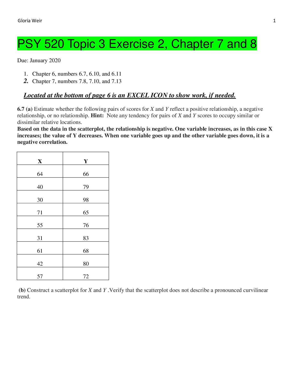
Exercise 3 PSY-520 6.7 (a) Estimate whether the following pairs of scores for X and Y reflect a positive relationship, a negative relationship, or no relationship. Hint: Note any tendency for pairs... f X and Y scores to occupy similar or dissimilar relative locations. There is a negative correlation for the following reasons; X and Y are on opposite sides of the mean, the higher X is the lower X is, as X increases Y decreases X and Y occupy difference areas for a plot or another way they are on opposite sides of the mean. (b) Construct a scatter plot for X and Y . Verify that the scatter plot does not describe a pronounced curvilinear trend. 20 30 40 50 60 70 80 60 65 70 75 80 85 90 95 100 X Y (c) Calculate r using the computation formula (6.1). X Values ∑ = 451 This study source was downloaded by 100000831988016 from CourseHero.com on 05-06-2022 04:18:18 GMT -05:00 https://www.coursehero.com/file/26883203/exericse3docx/ Mean = 50.111 ∑(X - Mx)2 = SSx = 1756.889 Y Values ∑ = 687 Mean = 76.333 ∑(Y - My)2 = SSy = 858 X and Y Combined N = 9 ∑(X - Mx)(Y - My) = -1122.333 R Calculation r = ∑((X - My)(Y - Mx)) / √((SSx)(SSy)) r = -1122.333 / √((1756.889)(858)) = -0.9141 6.10 On the basis of an extensive survey, the California Department of Education reported an r of - .32 for the relationship between the amount of time spent watching TV and the achievement test scores of schoolchildren. Each of the following statements represents a possible interpretation of this finding. Indicate whether each is true or false. (a) Every child who watches a lot of TV will perform poorly on the achievement tests. This is False for this to be true, it must be r = -1. (b) Extensive TV viewing causes a decline in test scores. True (c) Children who watch little TV will tend to perform well on the tests True (d) Children who perform well on the tests will tend to watch little TV. True (e) If Gretchen’s TV-viewing time is reduced by one-half, we can expect a substantial improvement in her test scores. False, there is no information to support this . (f) TV viewing could not possibly cause a decline in test scores. False, there is not information gathered to determine that tv viewing time could not cause a decline in test scores. 6.11 Assume that an r of .80 describes the relationship between daily food intake, measured in ounces, and body weight, measured in pounds, for a group of adults. Would a shift in the units of measurement from ounces to grams and from pounds to kilograms change the value of r ? Justify your answer. The answer would be no becsuse the formula to calculate R is the same regardless due to the fact that r does not have any units associated with it. R measures the correlation which measures the “degree” of liner association between two different variables. So when using the formula for the same two different variables as before but just different units the r results would be the same (Wittle & Wittle, 2013). This study source was downloaded by 100000831988016 from CourseHero.com on 05-06-2022 04:18:18 GMT -05:00 https://www.coursehero.com/file/26883203/exericse3docx/ r = Σ((X - Mx)(Y - My)) / √((SSx)(SSy)) = Σ((X - Mx)(Y - My)) / √((Σ(X - Mx)^2)(Σ(Y - My)^2)) If to change units of x to x’ = mx, and units of y to y’ = ny, then r’ = Σ((X’ - Mx’)(Y’ - My’)) / √((SSx’)(SSy’)) = Σ((X’ - Mx’)(Y’ - My’)) / √((Σ(X’ - Mx’)^2)(Σ(Y’ - My’)^2)) = Σ((mX - M(mx))(nY - M(ny)) / √((Σ(mX - M(mx))^2)(Σ(nY - M(ny))^2)) = (both numerator and denominator were multiplied by mn, and we can cancel it) = Σ((X - Mx)(Y - My)) / √((Σ(X - Mx)^2)(Σ(Y - My)^2)) = r Chapter 7, numbers 7.8, 7.10, and 7.13 7.8 Each of the following pairs represents the number of licensed drivers ( X ) and the number of cars ( Y ) for seven houses in my neighborhood: (a) Construct a scatter plot to verify a lack of pronounced curvilinearity This study source was downloaded by 100000831988016 from CourseHero.com on 05-06-2022 04:18:18 GMT -05:00 https://www.coursehero.com/file/26883203/exericse3docx/ 0.5 1 1.5 2 2.5 3 3.5 4 4.5 5 5.5 0 0.5 1 1.5 2 2.5 3 3.5 4 4.5 Driver (x) C a r s ( y ) . (b) Determine the least squares equation for these data. (Remember, you will first have to calculate r , SS y , and SS x .) X Values 5,5,2,2,3,1,2 Σ = 20 Mean = 2.85714 Σ(X - Mx)^2= SSx = 14.8571 Y Values 4,3,2,2,2,1,2 Σ = 16 Mean = 2.28571. Σ(Y - My)^2 = SSy = 5.42857 X and Y Combined. N = 7. Σ(X - Mx)(Y - My) = Sxy = 8.28571 R Calculation. r = Σ((X - Mx)(Y - My)) / √((SSx)(SSy)) = Σ((X - Mx)(Y - My)) / √((Σ(X - Mx)^2)(Σ(Y - My)^2)) = 0.922613 b1 = Sxy / SSx = 8.28571 / 14.8571 = 0.557694 b0 = My - b1 Mx = 2.28571 - 0.557694 * 2.85714 = 0.6923 y = b0 + b1 x = 0.6923 + 0.558445 x Fit curve is in scatterplot above. (c) Determine the standard error of estimate, s y | x , given that n 5 7. This study source was downloaded by 100000831988016 from CourseHero.com on 05-06-2022 04:18:18 GMT -05:00 https://www.coursehero.com/file/26883203/exericse3docx/ se = sqrt((SSy - b *Sxy)/(n - 2)) = sqrt((5.42857 - 0.557694*8.28571)/(7 - 2)) = 0.401915 (d) Predict the number of cars for each of two new families with two and five drivers. y(2) = 0.6923 + 0.558445*2 = 1.80919 y(5) = 0.6923 + 0.558445*5 = 3.48453 7.10 Assume that r 2 equals .50 for the relationship between height and weight for adults. Indicate whether the following statements are true or false. (a) Fifty percent of the variability in heights can be explained by variability in weights. True (b) There is a cause-effect relationship between height and weight. False due to there is no between the height and weight. (c) The heights of 50 percent of adults can be predicted exactly from their weights. False, it is 50 percent of the variability in height can be explained by variability in weights. (d) Fifty percent of the variability in weights is predictable from heights. True 7.13 In the original study of regression toward the mean, Sir Francis Galton noted a tendency for offspring of both tall and short parents to drift toward the mean height for offspring and referred to this tendency as “regression toward mediocrity.” What is wrong with the conclusion that eventually all heights will be close to their mean? If offspring’s were distributed randomly - that is, distribution the same as for present generation, then it will give the same picture: if parents are below median in height, then offspring would be with probability of 1/2 be either below, or above median in height, and this would be with higher probability above parents height than below. But overall distribution will be unchanged [Show More]

Last updated: 2 years ago

Preview 1 out of 5 pages