ISYE6501 Week 2 HW
Question 4.1 At my job we use clustering in an image system to understand the minerals that are
coming into our processing facility. Comparing the images to known mineral images, the system can
quan
...
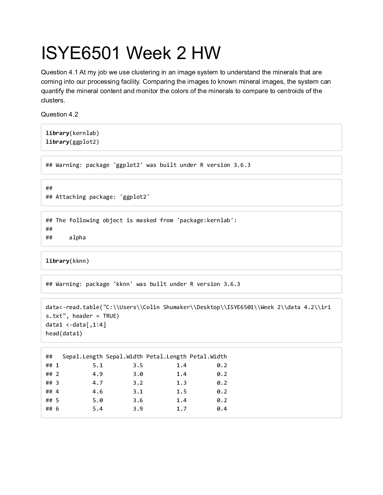
ISYE6501 Week 2 HW
Question 4.1 At my job we use clustering in an image system to understand the minerals that are
coming into our processing facility. Comparing the images to known mineral images, the system can
quantify the mineral content and monitor the colors of the minerals to compare to centroids of the
clusters.
Question 4.2
library(kernlab)
library(ggplot2)
## Warning: package 'ggplot2' was built under R version 3.6.3
##
## Attaching package: 'ggplot2'
## The following object is masked from 'package:kernlab':
##
## alpha
library(kknn)
## Warning: package 'kknn' was built under R version 3.6.3
data<-read.table("C:\\Users\\Colin Shumaker\\Desktop\\ISYE6501\\Week 2\\data 4.2\\iri
s.txt", header = TRUE)
data1 <-data[,1:4]
head(data1)
## Sepal.Length Sepal.Width Petal.Length Petal.Width
## 1 5.1 3.5 1.4 0.2
## 2 4.9 3.0 1.4 0.2
## 3 4.7 3.2 1.3 0.2
## 4 4.6 3.1 1.5 0.2
## 5 5.0 3.6 1.4 0.2
## 6 5.4 3.9 1.7 0.4species <-data[,5]
kvalues <- rep(0,10)
kx <- 1:10
set.seed(1000)
for (r in 1:10){
ktest <- kmeans(data1,r,nstart=5,iter.max = 10)
kx[r]<-r
kvalues[r]<-ktest$tot.withins
}
plot(kx,kvalues,type="b",xlab="Number of Clusters", ylab="Total Distance")
set.seed(4)
k <- kmeans(data1,3)
cat("Predictors 1,2,3,4","\n")
## Predictors 1,2,3,4
table(k$cluster,species)## species
## setosa versicolor virginica
## 1 0 48 14
## 2 0 2 36
## 3 50 0 0
set.seed(5)
k1 <- kmeans(data1[,1:3],3)
cat("Predictors 1,2,3","\n")
## Predictors 1,2,3
table(k1$cluster,species)
## species
## setosa versicolor virginica
## 1 0 45 13
## 2 50 0 0
## 3 0 5 37
set.seed(6)
k2 <- kmeans(data1[,2:4],3)
cat("Predictors 2,3,4","\n")
## Predictors 2,3,4
table(k2$cluster,species)
## species
## setosa versicolor virginica
## 1 0 48 5
## 2 50 0 0
## 3 0 2 45
set.seed(7)
k3 <- kmeans(data1[,c(1,2,4)],3)
cat("Predictors 1,2,4","\n")
## Predictors 1,2,4table(k3$cluster,species)
## species
## setosa versicolor virginica
## 1 0 39 15
## 2 0 11 35
## 3 50 0 0
set.seed(8)
k4 <- kmeans(data1[,c(1,3,4)],3)
cat("Predictors 1,3,4","\n")
## Predictors 1,3,4
table(k4$cluster,species)
## species
## setosa versicolor virginica
## 1 50 0 0
## 2 0 2 36
## 3 0 48 14
set.seed(9)
k5 <- kmeans(data1[,3:4],3)
cat("Predictors 3,4","\n")
## Predictors 3,4
table(k5$cluster,species)
## species
## setosa versicolor virginica
## 1 0 2 46
## 2 50 0 0
## 3 0 48 4
ggplot(data,aes(x=Petal.Length,y=Petal.Width, col=Species))+ geom_point()# best k value is 3 based on the plot to find the best combination of predictors. The
best accuracy is 96% showing that the best combination of predictors is 3 and 4. Evalu
ating the clusters using petal.length and petal.width shows the best response for spec
ies
Question 5.1
library(outliers)
data1<-read.table("C:\\Users\\Colin Shumaker\\Desktop\\ISYE6501\\Week 2\\data 5.1\\usc
rime.txt", header = TRUE)
crimesort <- t(data1$Crime[order(data1$Crime)])
plot(seq(1:length(crimesort)),crimesort,xlab="Sort", ylab="Crime Rates")grubbs.test(crimesort, type=10)
##
## Grubbs test for one outlier
##
## data: crimesort
## G = 2.81287, U = 0.82426, p-value = 0.07887
## alternative hypothesis: highest value 1993 is an outlier
[Show More]
