STAT 200 Week 6 Homework Problems, full solution guide, 100% correct.

Document Content and Description Below

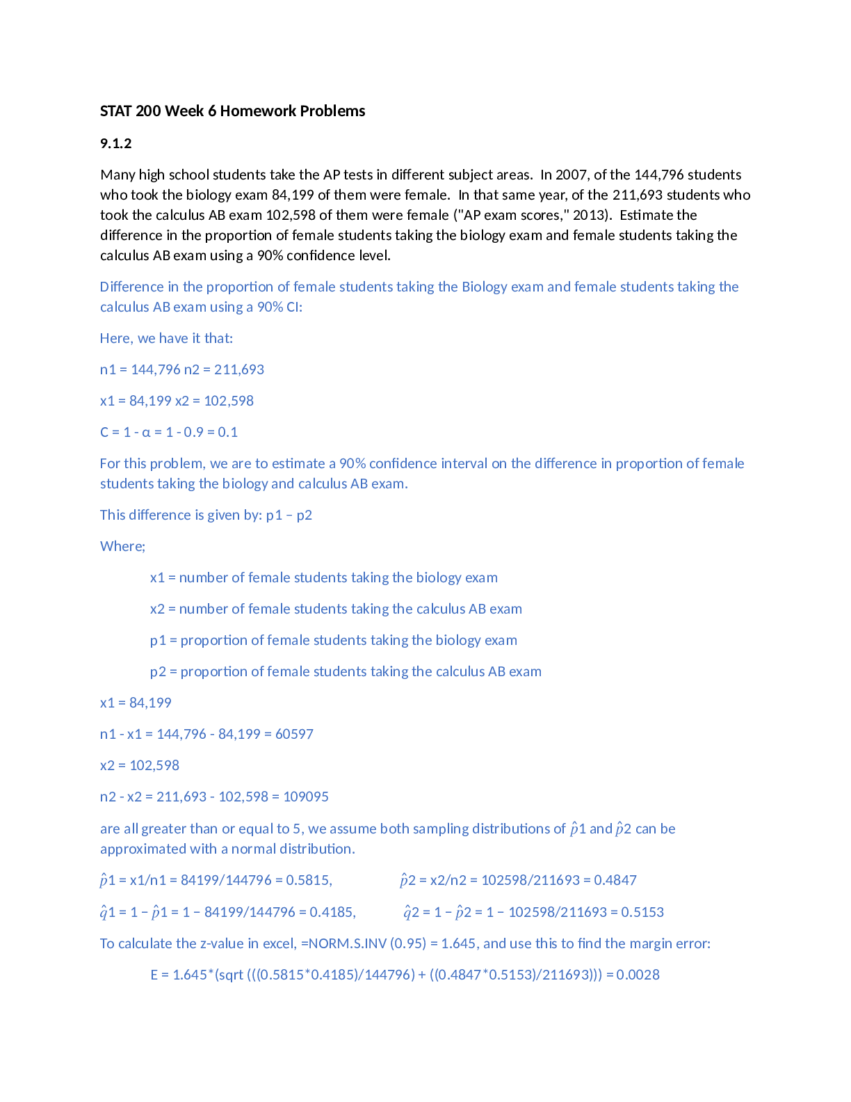
B exam 102,598 of them were female ("AP exam scores," 2013). Estimate the difference in the proportion of female students taking the biology exam and female students taking the calculus AB exam usin... g a 90% confidence level. Difference in the proportion of female students taking the Biology exam and female students taking the calculus AB exam using a 90% CI: Here, we have it that: n1 = 144,796 n2 = 211,693 x1 = 84,199 x2 = 102,598 C = 1 - α = 1 - 0.9 = 0.1 For this problem, we are to estimate a 90% confidence interval on the difference in proportion of female students taking the biology and calculus AB exam. This difference is given by: p1 – p2 Where; x1 = number of female students taking the biology exam x2 = number of female students taking the calculus AB exam p1 = proportion of female students taking the biology exam p2 = proportion of female students taking the calculus AB exam x1 = 84,199 n1 - x1 = 144,796 - 84,199 = 60597 x2 = 102,598 n2 - x2 = 211,693 - 102,598 = 109095 are all greater than or equal to 5, we assume both sampling distributions of �̂1 and �̂2 can be approximated with a normal distribution. �̂1 = x1/n1 = 84199/144796 = 0.5815, �̂2 = x2/n2 = 102598/211693 = 0.4847 �̂1 = 1 − �̂1 = 1 − 84199/144796 = 0.4185, �̂2 = 1 − �̂2 = 1 − 102598/211693 = 0.5153 To calculate the z-value in excel, =NORM.S.INV (0.95) = 1.645, and use this to find the margin error: E = 1.645*(sqrt (((0.5815*0.4185)/144796) + ((0.4847*0.5153)/211693))) = 0.0028 Then use it to compute the confidence interval on p1 - p2: (�1 − �̂2) − � < (�1 − �2) < (�̂1 − �̂2) + � (0.5815 − 0.4847) − 0.0028 < (�1 − �2) < (0.5815 − 0.4847) + 0.0028 �. �??� < (?� − ?�) < �. �??� Statistical Interpretation: There is a 90% chance that �. �??� < (?� − ?�) < �. �??� contains the true difference in proportions. Conclusion: The proportion of female students taking the biology exam is anywhere from 9.41% to 9.96% higher than the proportion of female students taking the calculus AB exam. 9.1.5 Are there more children diagnosed with Autism Spectrum Disorder (ASD) in states that have larger urban areas over states that are mostly rural? In the state of Pennsylvania, a fairly urban state, there are 245 eight year olds diagnosed with ASD out of 18,440 eight year olds evaluated. In the state of Utah, a fairly rural state, there are 45 eight year olds diagnosed with ASD out of 2,123 eight year olds evaluated ("Autism and developmental," 2008). Is there enough evidence to show that the proportion of children diagnosed with ASD in Pennsylvania is more than the proportion in Utah? Test at the 1% level. Testing at 1% level of significance: Here, we have it that; n1 = 18,440 n2 = 2,123 x1 = 245 x2 = 45 α = 0.01 For this problem, we are testing whether the proportion of children diagnosed with ADS in Pennsylvania is more than that of Utah. Where; x1 = number of children diagnosed with Autism Spectrum Disorder (ASD) in Pennsylvania x2 = number of children diagnosed with ASD in Utah p1 = proportion of children diagnosed with ASD in Pennsylvania p2 = proportion of children diagnosed with ASD in Utah The hypothesis will be: H0 : p1 = p2 Vs. H1 : p1 > p2 x1 = 245 n1 - x1 = 18440 -245 = 18195 x2 = 45 n2 - x2 = 2123 - 45 = 2078 are all greater than or equal to 5, we assume both sampling distributions of �̂1 and �̂2 can be approximated with a normal distribution. �̂1 = �1/�1 = 245/18144 = 0.0133, �̂2 = �2/�2 = 45/2123 = 0.0212 �̂1 = 1 − �̂1 = 1 − 245/18144 = 0.9867, �̂2 = 1 − �̂2 = 1 − 45/2123 = 0.9788 Then compute the pooled proportions, �̅ = (245 + 45) / (18144 + 2123) = 0.0141 and �̅ = 1 – 0.0141 = 0.9859 the test statistic z = -2.927 Conclusion Since the p-value is greater than the level of significance (i.e. [p-value = 0.9983] > [α = 0.01]), we fail to reject ?�. This is not enough evidence to show that the proportion of children diagnosed with ASD in Pennsylvania is more than the proportion of children diagnosed with ASD in Utah. 9.2.3 All Fresh Seafood is a wholesale fish company based on the east coast of the U.S. Catalina Offshore Products is a wholesale fish company based on the west coast of the U.S. Table #9.2.5 contains prices from both companies for specific fish types ("Seafood online," 2013) ("Buy sushi grade," 2013). Do the data provide enough evidence to show that a west coast fish wholesaler is more expensive than an east coast wholesaler? Test at the 5% level. Table #9.2.5: Wholesale Prices of Fish in Dollars Fish All Fresh Seafood Prices Catalina Offshore Products Prices Cod 19.99 17.99 Tilapi 6.00 13.99 Farmed Salmon 19.99 22.99 Organic Salmon 24.99 24.99 Grouper Fillet 29.99 19.99 Tuna 28.99 31.99 Swordfish 23.99 23.99 Sea Bass 32.99 23.99 Striped Bass 29.99 14.99 Testing at 5% level of significance: We have that; n = 9 α = 0.05 For this problem, we are testing whether a west coast fish wholesaler is more expensive than an east coast wholesaler. Where; x1 = wholesale prices from west coast fishery x2 = wholesale prices from east coast fishery μ1 = mean wholesale prices from west coast fishery μ2 = mean wholesale prices from east coast fishery the hypothesis will be; H0: �1 = �2 Vs. H1: �1 > �2 at � = 0.05 Thus �̅= $2.446 and s� = $7.399, where �̅ is the sum of the difference between x1 and x2 divided by n and sd is the standard deviation of the difference. Thus t = (2.446 – 0) / (7.399/ sqrt(9)) = 0.9915 We can get the p- value in excel by: =1 - T.DIST(0.9915, 9-1, TRUE) = 0.175 Conclusion Since the p-value is greater than the level of significance (i.e. [p-value = 0.175] > [α = 0.05]), we fail to reject ?�. There is not enough evidence to show that west coast fish wholesalers are more expensive than east coast wholesalers. 9.2.6 The British Department of Transportation studied to see if people avoid driving on Friday the 13th. They did a traffic count on a Friday and then again on a Friday the 13th at the same two locations ("Friday the 13th," 2013). The data for each location on the two different dates is in table #9.2.6. Estimate the mean difference in traffic count between the 6th and the 13th using a 90% level. Table #9.2.6: Traffic Count Dates 6th 13th 1990, July 139246 138548 1990, July 134012 132908 1991, September 137055 136018 1991, September 133732 131843 1991, December 123552 121641 1991, December 121139 118723 1992, March 128293 125532 1992, March 124631 120249 1992, November 124609 122770 1992, November 117584 117263 Difference in traffic count between the 6th and the 13th using a 90% level: n = 10 given that these are “paired” samples, the values for n1 = n2. C = 1 - α = 1 - 0.9 = 0.1 For this problem, we are to estimate a 90% confidence interval on the difference in the paired samples of traffic counts on Friday the 6th and Friday the 13th. This difference is given by: d = x1 – x2. Where; x1 = traffic count on Friday the 6th x2 = traffic count on Friday the 13th µ1 = mean traffic count on Friday the 6th µ2 = mean traffic count on Friday the 13th mean (�̅) = 1835.8 and sd = 1176.0139 we can get the t-value by: =T.INV.2T (0.1, 10-1) = 1.833, from excel. E = 1.833(1176.01/sqrt (10)) = 681.7 �̅− � < �� < �̅+ � 1835.8 − 681.7 < �� < 1835.8 + 681.7 ��??. � < ?� < �?��. ? Statistical Interpretation: There is a 90% chance that ��??. � < ?� < �?��. ? contains the true difference in traffic counts. The mean difference in traffic counts between Friday the 6th and Friday the 13th is between 1154.1 and 2517.5. 9.3.1 The income of males in each state of the United States, including the District of Columbia and Puerto Rico, are given in table #9.3.3, and the income of females is given in table #9.3.4 ("Median income of," 2013). Is there enough evidence to show that the mean income of males is more than of females? Test at the 1% level. Table #9.3.3: Data of Income for Males $42,951 $52,379 $42,544 $37,488 $49,281 $50,987 $60,705 $50,411 $66,760 $40,951 $43,902 $45,494 $41,528 $50,746 $45,183 $43,624 $43,993 $41,612 $46,313 $43,944 $56,708 $60,264 $50,053 $50,580 $40,202 $43,146 $41,635 $42,182 $41,803 $53,033 $60,568 $41,037 $50,388 $41,950 $44,660 $46,176 $41,420 $45,976 $47,956 $22,529 $48,842 $41,464 $40,285 $41,309 $43,160 $47,573 $44,057 $52,805 $53,046 $42,125 $46,214 $51,630 Table #9.3.4: Data of Income for Females $31,862 $40,550 $36,048 $30,752 $41,817 $40,236 $47,476 $40,500 $60,332 $33,823 $35,438 $37,242 $31,238 $39,150 $34,023 $33,745 $33,269 $32,684 $31,844 $34,599 $48,748 $46,185 $36,931 $40,416 $29,548 $33,865 $31,067 $33,424 $35,484 $41,021 $47,155 $32,316 $42,113 $33,459 $32,462 $35,746 $31,274 $36,027 $37,089 $22,117 $41,412 $31,330 $31,329 $33,184 $35,301 $32,843 $38,177 $40,969 $40,993 $29,688 $35,890 $34,381 Testing at 1% level: We have that; �1 = 52; �2 = 52 α = 0.01 For this problem, we are testing whether income of males is more than income of females. Where; x1 = income of a male in 2013 x2 = income of a female in 2013 µ1 = mean income of a male in 2013 µ2 = mean income of a female in 2013 the hypothesis is: �0: �1 = �2 Vs. �1: �1 > �2 at � = 0.01 To compute the sample statistic, we first need to compute the mean and standard deviation for each data set. These are given by: �̅1 = $46,453.31, �1 = $7,030.71 �̅2 = $36,511.00, �2 = $6,138.12 �1 2 = 7030.712 = 49,430,918.45 �2 2 = 6138.122 = 37,676,539.45 For this problem, we have: =1-F.DIST (49,430,918.45/37,676,539.45, 52-1, 52-1, TRUE) = 0.1677 Thus 0.1677 > 0.05, we can assume variances are equal (i.e. �12 = �22) Since the variances are equal (i.e. �12 = �22), so we need to compute the pooled standard deviation: sp = 6599.5 The t statistic is given by: 7.682, df = 102 =T.DIST (7.682, 102, TRUE)” = 4.963 * 10-12 Conclusion Since the p-value is less than the level of significance (i.e. [p-value = 4.963 * 10-12] < [α = 0.01]), we reject ?0. This is enough evidence to show that the mean income of males is more than of females [Show More]

Last updated: 2 years ago

Preview 1 out of 15 pages