Computer Architecture > QUESTIONS & ANSWERS > CS 189 Introduction to Machine Learning Homework 6 | University of California (All)
CS 189 Introduction to Machine Learning Homework 6 | University of California
Document Content and Description Below
CS 189 Introduction to Machine Learning Spring 2021 Jonathan Shewchuk HW6 Due: Wednesday, April 21 at 11:59 pm Deliverables: 1. Submit your predictions for the test sets to Kaggle as early as poss... ible. Include your Kaggle scores in your write-up (see below). The Kaggle competition for this assignment can be found at • https://www.kaggle.com/c/spring21-cs189-hw6-cifar10 2. The written portion: • Submit a PDF of your homework, with an appendix listing all your code, to the Gradescope assignment titled “Homework 6 Write-Up”. Please see section 3.3 for an easy way to gather all your code for the submission (you are not required to use it, but we would strongly recommend using it). • In addition, please include, as your solutions to each coding problem, the specific subset of code relevant to that part of the problem. Whenever we say “include code”, that means you can either include a screenshot of your code, or typeset your code in your submission (using markdown or LATEX). • You may typeset your homework in LaTeX or Word (submit PDF format, not .doc/.docx format) or submit neatly handwritten and scanned solutions. Please start each question on a new page. • If there are graphs, include those graphs in the correct sections. Do not put them in an appendix. We need each solution to be self-contained on pages of its own. • In your write-up, please state with whom you worked on the homework. • In your write-up, please copy the following statement and sign your signature next to it. (Mac Preview and FoxIt PDF Reader, among others, have tools to let you sign a PDF file.) We want to make it extra clear so that no one inadvertently cheats. “I certify that all solutions are entirely in my own words and that I have not looked at another student’s solutions. I have given credit to all external sources I consulted.” 3. Submit all the code needed to reproduce your results to the Gradescope assignment entitled “Homework 6 Code”. Yes, you must submit your code twice: in your PDF write-up following the directions as described above so the readers can easily read it, and once in compilable/interpretable form so the readers can easily run it. Do NOT include any data files we provided. Please include a short file named README listing your name, student ID, and instructions on how to reproduce your results. Please take care that your code doesn’t take up inordinate amounts of time or memory. If your code cannot be executed, your solution cannot be verified. HW6, 'UCB CS 189, Spring 2021. All Rights Reserved. This may not be publicly shared without explicit permission. 11 Honor Code Declare and sign the following statement: “I certify that all solutions in this document are entirely my own and that I have not looked at anyone else’s solution. I have given credit to all external sources I consulted.” Signature : While discussions are encouraged, everything in your solution must be your (and only your) creation. Furthermore, all external material (i.e., anything outside lectures and assigned readings, including figures and pictures) should be cited properly. We wish to remind you that consequences of academic misconduct are particularly severe! 2 Background This section will provide a background on neural-networks that is designed to help you complete the assignment. There are no questions in this part. The questions for the homework begin in section 4. 2.1 Neural Networks Many of the most exciting recent breakthroughs in machine learning have come from “deep” (read: manylayer) neural networks, such as the deep reinforcement learning algorithm that learned to play Atari from pixels, or the GPT-2 model, which generates text that is nearly indistinguishable from human-generated text. Neural network libraries such as Tensorflow and PyTorch have made training complicated neural network architectures very easy. However, we want to emphasize that neural networks begin with fundamentally simple models that are just a few steps removed from basic logistic regression. In this assignment, you will build two fundamental types of neural network models, all in plain numpy: a feed-forward fully-connected network, and a convolutional neural network. We will start with the essential elements and then build up in complexity. A neural network model is defined by the following. • An architecture defining the flow of information between computational layers. This defines the composition of functions that the network performs from input to output. • A cost function (e.g. cross-entropy or mean squared error). • An optimization algorithm (e.g. stochastic gradient descent with backpropagation). • A set of hyperparameters (e.g. learning rate, batch size, etc.). Each layer is defined by the following components. • A parameterized function that defines the layer’s map from input to output (e.g. f (x) = σ(W x + b)). • An activation function σ (e.g. ReLU, sigmoid, etc.). • A set of parameters (e.g. weights and biases). Neural networks are commonly used for supervised learning problems, where we have a set of inputs and a set of labels, and we want to learn the function that maps inputs to labels. To learn this function, we need HW6, 'UCB CS 189, Spring 2021. All Rights Reserved. This may not be publicly shared without explicit permission. 2to update the parameters of the network (the weights and biases). We do this using mini-batch gradient descent. In order to compute the gradients for gradient descent, we will use a dynamic programming algorithm called backpropagation. In the backpropagation algorithm, we first compute what is called a “forward pass” of the network. In the forward pass, we send a mini-batch of input data (e.g. 50 datapoints) through the network. The result is a set of outputs, which we use to compute our loss function. We then take the derivatives of this loss with respect to the parameters of each layer, starting with the output of the network and using the chain rule to propagate backwards through the layers. This is called the “backward pass.” During the backward pass we compute the derivatives of the loss function with respect to each of the model parameters, starting from the last layer and “propagating” the information from the loss function backwards through the network. This lets us calculate derivatives with respect to all the parameters of our network while letting us avoid computing the same derivatives multiple times. To summarize, training a neural network involves three steps. 1. Forward propagation of inputs. 2. Computing the cost. 3. Backpropagation and parameter updates. 2.2 Batching When Building neural networks, we have to carefully consider the data. In homework 4, you coded both batch gradient descent and stochastic gradient descent for logistic regression. For the stochastic version, where only a single data point was used, the form of derivatives used in gradient descent were different than those of batch gradient descent. Neural-networks always operate on mini-batches, or subsets of the data matrix. This is because operating on all the data at once would be impossible given current compute and actually bad for optimization, while operating on a single data point would be far too noisy. Thus, every step of your neural network must be defined to operate on batches of data. For example, the input to a fully connected neural network would be a matrix of shape (B; d) where B is the batch size and d is the number of features. The input to a convolutional neural network would be a tensor of shape (B; H; W; C) where B is the batch size, H is the height of the image, W is the width of the image, and C is the number of channels in the image (3 for RGB). Because you are writing the gradient descent algorithm to work on mini-batches, all of your derivations must work for mini-batches as well. This is important to keep in mind as you complete this assignment, and many of the derivations may be different than those you have seen in class. Thinking in terms of mini-batches often changes the shapes and operations you do. Your derivations must be for mini-batches and cannot use for loops to iterate over individual data points. This is one aspect of the assignemnt that students often find to be very difficult. 2.3 Feed-Forward, Fully-Connected Neural Networks A feed-forward, fully-connected neural network layer performs an affine transformation of an input, followed by a nonlinear activation function. We will use the following notation when defining fully-connected layers, with superscripts surrounded by brackets indexing layers and subscripts indexing the vector/matrix elements. • x: A single data vector, of shape 1 × d, where d is the number of features. HW6, 'UCB CS 189, Spring 2021. All Rights Reserved. This may not be publicly shared without explicit permission. 3ŷ W[0] W[1] W[2] b[0] b[1] b[2] x h[0] h[1] Figure 1: A 3-layer fully-connected neural network. d∑i=0 xi W[0] ij + bj[0] σ[0]( ⋅ ) W 0,j b[0] j h[0] j x1 W1,j W 2,j x0 x2 Figure 2: A single fully-connected neuron. • y: A single label vector, of shape 1×k, where k is the number of classes (for a classification problem), or the number of output features (for a regression problem). • n[l]: The number of neurons in layer l. • W[l]: A matrix of weights connecting layer l − 1 with layer l, of shape n[l−1] × n[l]. At layer 0, it is shape d × n[l]. • b[l]: The bias vector for layer l, of shape 1 × n[l]. • h[l]: The output of layer l. This is a vector of shape 1 × n[i]. • σ[l](·): The nonlinear “activation function” applied at layer l. A fully-connected layer l is a function φ[l](h[l−1]) = σ[l](h[l−1]W[l] + b[l]) = h[l]: At layer 0, h[l−1] is simply the data vector x. We will use the term z[l] = h[l−1]W[l] + b[l] as shorthand for the intermediate result within layer l before applying the activation function σ. Each layer is computed sequentially and the output of one layer is used as the input to the next. A neural network is thus a composition of functions. We want to find the parameters of the function that takes us from our input examples x to our labels y. When used for classifiation, feed forward networks accept inputs as d-dimensional vectors, and the labels will be k-dimensional ”one-hot” vectors, where k is the number of classes. A one-hot vector is a binary vector whose elements are computed according to the following function: yi = 8>>><>>>: 1 x 2 class i; 0 otherwise. For example, for a classification problem with 3 classes, the label encoding an example from class 2 (zeroindexing) would be: [0; 0; 1]. HW6, 'UCB CS 189, Spring 2021. All Rights Reserved. This may not be publicly shared without explicit permission. 42.4 Convolutional Neural Networks We will use the following notation when defining a convolutional neural network layer. • X: A single image tensor, of shape 1 × d1 × d2 × c, where d1 and d2 are the spatial dimensions, and c is the number of channels. • y: A single label vector, of shape 1 × k, where k is the number of classes. • n[l]: The number of neurons in layer l. • (k1; k2)[l]: The size of the spatial dimensions of the filters in layer l. Also referred to as the kernel1 size. • W[l]: The tensor of filters convolved at layer l. This tensor has shape k1 × k2 × n[l−1] × n[l]. • b[l]: The bias vector for layer l, of shape 1 × n[l]. • H[l]: The output of layer l. This is a tensor of shape 1 × r1 × r2 × n[l], where (r1; r2) is the shape of output of the convolution operation. Below we will discuss how to calculate this. • σ[l](·): The nonlinear “activation function” applied at layer l. In a convolutional layer, each filter is convolved with the input image, across every image channel. This operation is, essentially, a sliding sum of element-wise products. Figure 3 gives a visual example. To compute a single element in the intermediate output Z, for a single neuron n and a single channel c in the input X, we compute Z[d1; d2; n] = (X ∗ W)[d1; d2; n] = X i Xj Xc W[i; j; c; n]X[d1 + i; d2 + j; c] + b[n]: Please note that the formula above is the cross-correlation formula from signal processing and NOT the convolution formula. Nevertheless this is what ML people call convolution and so will we. It actually makes sense to use cross-correlation instead of using convolution because the former can be interpreted as producing an output which is higher at locations where the image has the pattern in the filter and low elsewhere. Furthermore, convolution is the same as cross-correlation with a flipped filter, and we learn the filters, so it should not make any difference operationally whether you implement convolution or cross-correlation. However, in order to pass the tests, you must implement cross-correlation and call that convolution because that’s how we do it in ML-land. In this equation, we drop the layer superscripts for clarity, and index elements of the matrices in brackets. The output of this operation is what we call a “feature map,” which essentially captures the strength of each filter at every region in the image. In the equation above, we slide the filter over the image in increments of one pixel. We can choose to take a larger steps instead. The size of the step taken in the convolution operation is referred to as the stride. [Show More]
Last updated: 4 months ago
Preview 4 out of 26 pages

Loading document previews ...
Buy this document to get the full access instantly
Instant Download Access after purchase
Buy NowInstant download
We Accept:

Reviews( 0 )
$8.00
Can't find what you want? Try our AI powered Search
Document information
Connected school, study & course
About the document
Uploaded On
Apr 20, 2023
Number of pages
26
Written in

Additional information
This document has been written for:
Uploaded
Apr 20, 2023
Downloads
0
Views
73