The article “Obesity prevalence and the local food environment” studies 1295
adults and the affiliation of obesity in areas of healthy food markets compared to areas of fast
food and small grocery stores in the souther
...
The article “Obesity prevalence and the local food environment” studies 1295
adults and the affiliation of obesity in areas of healthy food markets compared to areas of fast
food and small grocery stores in the southern region of the United States. (Morland and Evenson,
2008, p.1) Their research questions asked if there actually is an association of obesity in areas of
healthy and unhealthy food restaurants, if distance contributed, age, as well as socioeconomic
and race/ethnic status. They hypothesized that the more supermarkets of high nutrition food and
less fast food and small grocery stores would contain a population of lower obesity. Overall,
living closer to a supermarket would result in a lower BMI compared to those who live closer to
a fast food restaurant. (Morland and Evenson, 2008, p.2)
This is an observational study, “the sample population being studied is measured, or
surveyed, as it is. The researcher observes the subjects and measures variables, however does not
influence the population in any way or attempt to intervene in the study.” (wikipedia.com) There
is no manipulation by the researcher. “A random digit dialed phone survey of the noninstitutionalized adult population in two distinct geographic locations was conducted. 1295
adults were chosen.” (Moreland and Evenson, 2008) They did not force people to be obese or to
spend money at a grocery store or fast food restaurant.
One method used was sample population. “A sampling company (Genesys Marketing
Systems Group) provided a listing of residential household phone numbers, while Clearwater
Research, Inc. (Boise, Idaho), conducted the telephone surveys. (2009) Business addresses of
places where people could obtain food were collected from the local Departments of
Environmental Health and state Departments of Agriculture in 2006. The 1997 North America
Industry Classification System codes and definitions were modified to describe the types of food
stores and food service places located in each census tract.” (Moreland and Evenson, 2008)
This study source was downloaded by 100000796615030 from CourseHero.com on 07-18-2021 07:50:56 GMT -05:00
https://www.coursehero.com/file/33817211/obesity-2docx/
This study resource was
shared via CourseHero.com
Obesity prevalence
3
Another method used was Source population using an adult population. These methods
are appropriate because the Sample population is only being surveyed and no manipulation is
noted. The survey was done during the weekday, weeknight and weekend hours. The respondents
were randomly chosen. They tried to include everyone. They tried to cover all areas of the
experiment that are needed to get accurate findings.
Data collected was Quantitative. Quantitative data basically involves descriptive data,
such as survey data and observational data. “Table 1. Mean age was 48, 64.7% were women.
23.5% had graduated college. Table 2 The prevalence of obesity was lowered by 0.73 in areas
that had at least one supermarket. In table 3 Each mile closer to a supermarket had a 6% higher
prevalence of obesity. Obesity was defined at greater than 30 kg/m². The researchers applied the
descriptive statistical analysis approach in connection to the USDA recommended score
measurement.” (Chen, Jaenicke, & Volpe, 2016; Morland & Evenson, 2009).
One weakness is limiting factors. They included only two geographical areas to
investigate. The response rates were low, “Overall 20.2%, Forsyth County 24.0% Winston-Salem
24.5% and Jackson 16.69%.” Also, selection bias may have occurred as the survey respondents
tended to be highly educated. Only landlines were used in the data, people with only cell phones
are not included in the data. Another weakness is that Height and weight are self-reported and
BMI’s may not be correct. One exclusion would be that the study does not include 1-5-year old’s.
Analysis methods are showing in table 1-3. Some Data Analysis methods used was
“Census tracts based of the 2000 US Census, 2000 US Census of Population and Housing
Summary, Department of Environmental Health and state Departments of Agriculture. ArcGIS
software was used for distances.” Descriptive analysis was used describing the study population.
This is not appropriate because it only used 2 geographical areas. The food environment data
This study source was downloaded by 100000796615030 from CourseHero.com on 07-18-2021 07:50:56 GMT -05:00
https://www.coursehero.com/file/33817211/obesity-2docx/
This study resource was
shared via CourseHero.com
Obesity prevalence
4
was collected 3 years after the individual-level data. “Table 1 Average Distance to nearest
supermarket 1.77 miles compared to distance to nearest fast food 1.39 miles.”
“Another Weakness is distance results between home and supermarket or home and fast
food were not in the direction hypothesized.” “The research was based on the density of stores
within a census tract and assumes that all residents within the census tract (regardless of where
they are located) have a similar exposure. It is possible, and in fact likely, that some of the people
living in the residential census tract where exposure was assigned do not actually shop in that
area.” “Some components not touched in this study is Transportation, mobility, and other factors.
“We calculated individuals’ body mass indexes (BMIs; defined as weight in kilograms divided by
the square of height in meters) on the basis of IRi household members’ self-reported weights and
heights ([weight in pounds/(height in inches)2] · 703). On the basis of our BMI calculations, we
constructed indicator variables for obesity and overweight status using different criteria for
adults and children.” (American Journal of Public Health pg. 882.) They performed the statistical
analysis using Stata version 13 (StataCorp LP, College Station, TX.) The weakness is that the
data sampling is not big enough absolutely prove that being inside or outside of a food desert
area is what was specifically causing obesity. “Almost all the individual-level demographics and
lifestyle choices were significantly associated with obesity or overweight status. Specifically, age
was positively associated with obesity or overweight status, and being female was negatively
associated with obesity or overweight status. A higher diet feature score was related to a higher
probability of being obese or overweight, which was expected if individuals adopted special diets
(low-fat, low-sugar, low-salt, etc.) when concerned about their weight or BMI.” (American
Journal of Public Health pg. 884, 885.)
Key demographics included age, gender, race/ethnicity, education and employment.
Height and weight are self-reported. 38,650 participants from 18,381 households within 2,104
This study source was downloaded by 100000796615030 from CourseHero.com on 07-18-2021 07:50:56 GMT -05:00
https://www.coursehero.com/file/33817211/obesity-2docx/
This study resource was
shared via CourseHero.com
Obesity prevalence
5
U.S. counties. “Using the USDA Score, researchers analyzed the adherence of monthly
expenditure per household of 24 aggregated food categories as recommended by the US
Department of Agriculture Food Plans among other chosen government organizations.”
The results were that “Neighborhood food environment factors were examined in the
context of the obesity status even in the presence of controlled home food environment factors
The USDA Score was negatively correlated with the obesity status. A 1-point increase in average
USDAScore would decrease the odds of obesity status by about 7% (odds ratio [OR]=0.93; 95%
confidence interval [CI]=0.90, 0.96). Based on estimates of parameters from this model, we
predicted the average probabilities of obesity with increasing levels of USDAScores by gender.
The estimated probability of obesity for individuals living in households with the highest
USDAScores (USDAScore=13) was about 0.15 lower than for those in households with the
lowest USDAScores (USDAScore=1). Additional analysis indicated that county-level obesity
rates were negatively correlated with average USDAScores at the county level (Pearson
correlation coefficient=–0.12; P<.001). County-level poverty rates were not significantly
associated with obesity or overweight status. Living in metropolitan counties was significantly
associated with lower odds of being obese. The tract-level food desert indicator was positively
associated with obesity or overweight. With other factors remaining constant, a census tract–
level switch from a non–food desert to a food desert increased an individual’s odds of being
obese by about 30% (OR=1.30; 95% CI=1.06, 1.59) and of being overweight by about 19%
(OR=1.19; 95% CI=1.02, 1.38).” (American Journal of Public Health pg. 885) In essence this is
saying if you live in a desert track you are more likely to be obese.
Some Differences in results include self-reporting height and weight, scanning devices,
home to store and home to fast food to name a few. Another difference to take note of is the
difference in calculating the data in Tables 1-3. In Table 1 and 2 they use the percentage to find
This study source was downloaded by 100000796615030 from CourseHero.com on 07-18-2021 07:50:56 GMT -05:00
https://www.coursehero.com/file/33817211/obesity-2docx/
This study resource was
shared via CourseHero.com
Obesity prevalence
6
the mean and standard deviation. What this means is in Table 2 could be part of a statistical
inference or drawing conclusions about the entire population. In Table 3 they use the 95%
confidence interval for their demographics which means they estimated a predetermined chance
of capturing the value of the population.
Some limitations are inconsistent choice of measurement variables from the chosen ones
by previous scholars. The varied choice of variables resulted into the inconsistency of effects and
efforts in each case. “Measurement of food available at home is labor intensive and constrained
by the duration of data collection.” The time factor, food frequency questionnaires and the 24-
hour recalls have the considerable measurement errors with bias being higher for food frequency
questionnaires. There were numerous variables to be tested, which required additional efforts and
time. Another limitation is most of the study was from the Census Bureau’s American
Community Survey from 2010-2012 and the USDA to get their demographics and statistics. This
hindered the project because not everyone could have answered or answered honestly. The
researchers are trying to get an estimate on the population, obtain information easier, and predict
some of the results. The disadvantage is that the study wasn’t as randomized or as accurate as it
could have been.
Major conclusions form the study are that living closer to a supermarket would result in a
lower BMI 0.73% compared to those who live closer to a fast food restaurant 1.36%. In the
reference article the conclusions were one third of sample was overweight 31.92% and one third
were obese 31.54%. Depending on where you live you have a higher chance of being obese. That
the closer you live to a grocery store the less likely you are to being overweight. Being closer to
fast food means your chances of being overweight or having a larger BMI are higher.
In the Article Obesity prevalence, it focuses more on neighborhoods with grocery stores
and markets to neighborhoods with more fast food restaurants and less grocery stores. The article
[Show More]









![Preview of FDSC 1133 Exam 1 [Food Science Fundamentals] 140 Questions & 100% Verified Answers Grade A](https://browseimages.nyc3.digitaloceanspaces.com/paper-images/2026/04/01/znnLS2iB2026-04-01-01-4869cc4f56594bb.png)