University of California, Los Angeles LIFESCIENC 30A. LS 30A-1 Homework 10 Solutions. Total points: 68. from December 2019

Document Content and Description Below

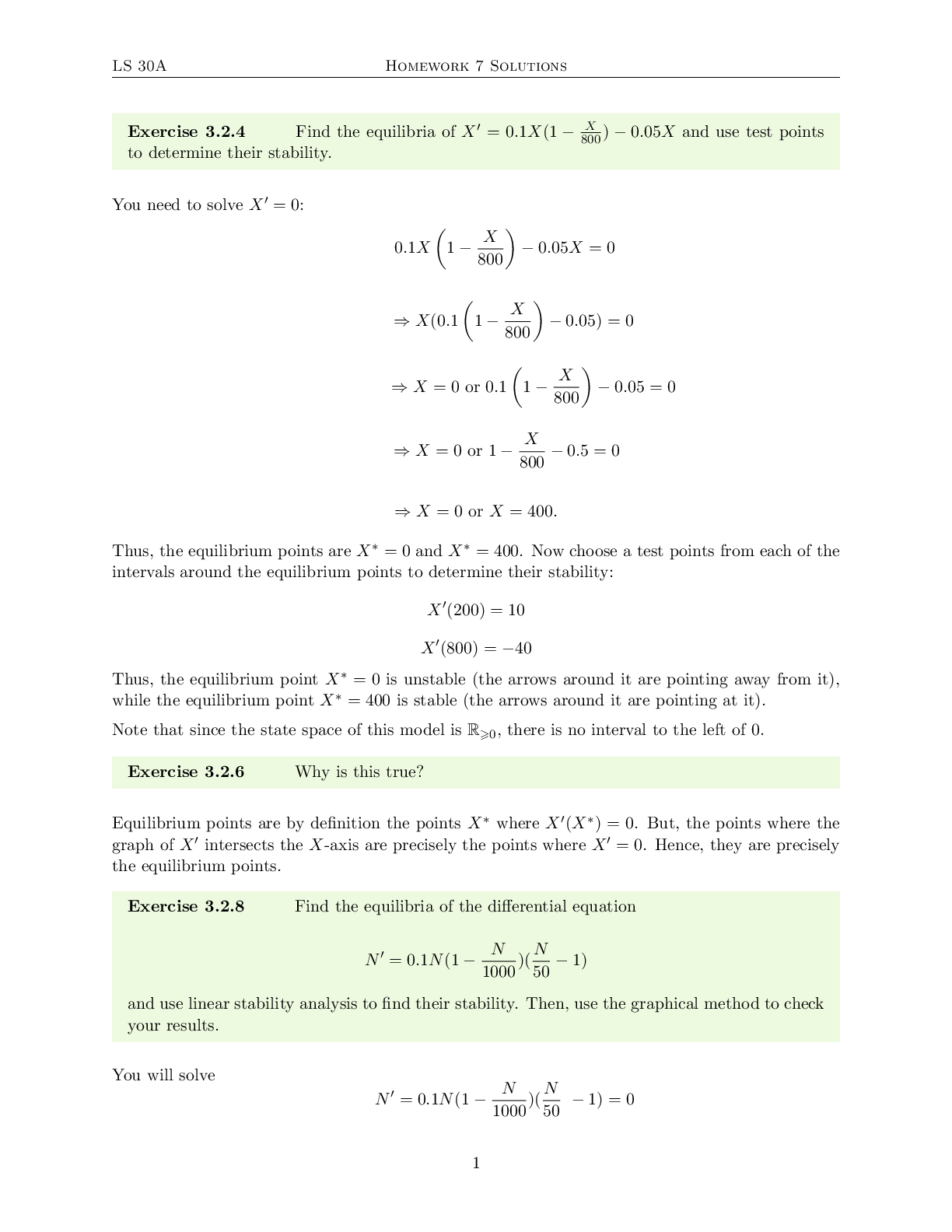
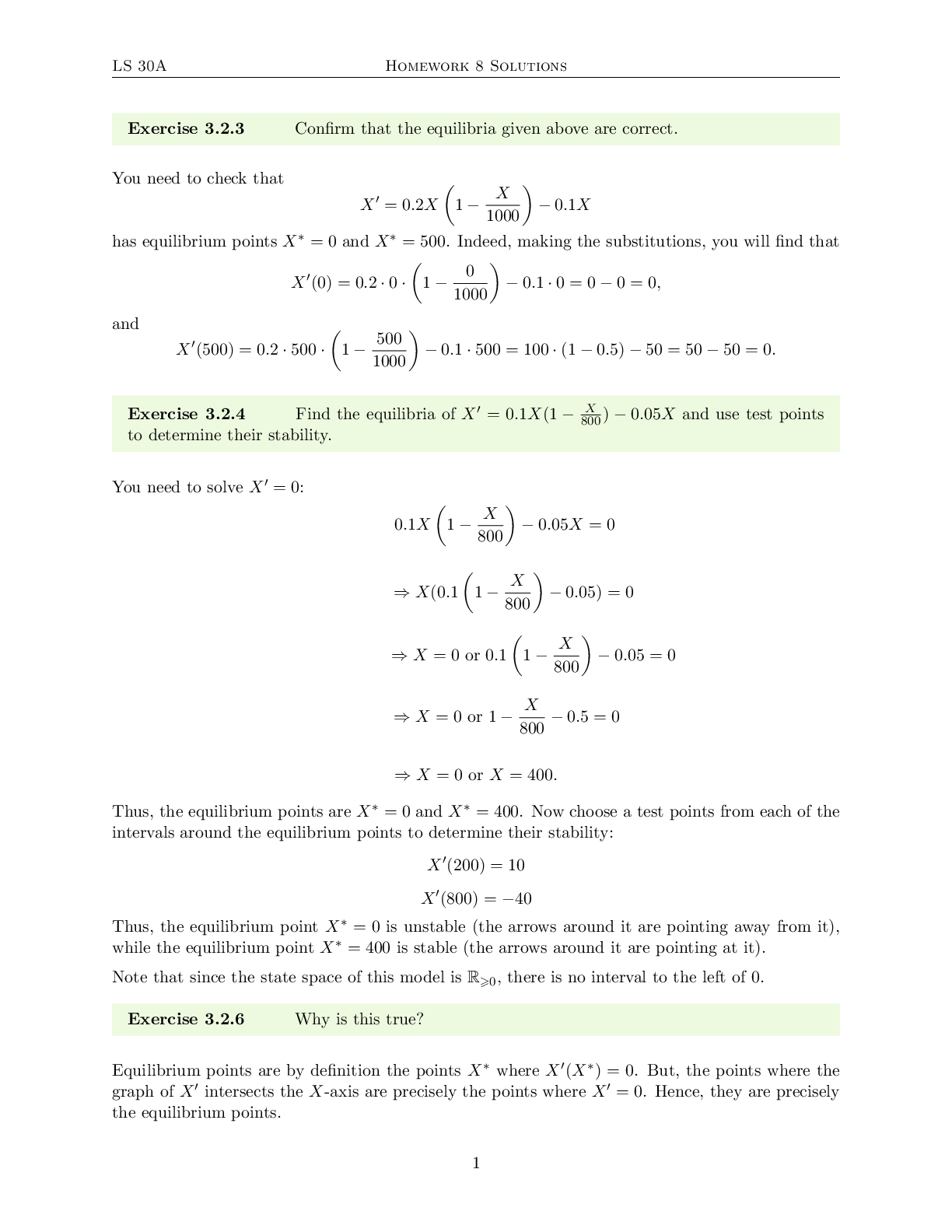
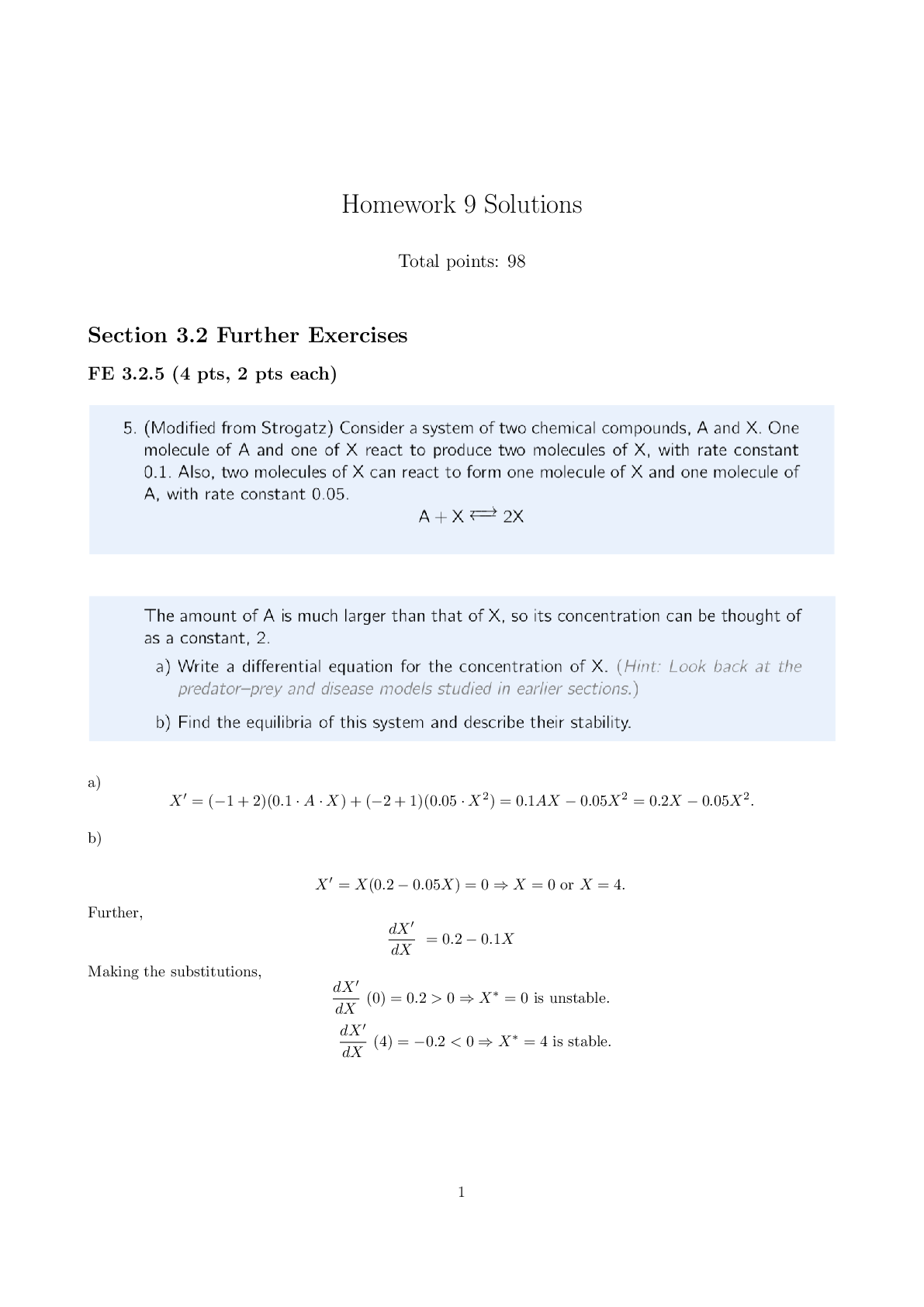
Homework 10 Solutions Total points: 68 December 2019 Section 3.2 Further Exercises Section 3.4 Further Exercises + 10 FE 3.4.3 (2 pts) (0; 0): saddle point; (5000; 0): saddle point; (1; 9... :998): stable spiral NOTE It is not easy to read off the stabilities from the vector field plots. However, if you study them at many different levels of magnification, you can tell that (0; 0) and (5000; 0) are definitely saddle points. As you are exploring these points, it helps to allow negative values for the state variables (even if such values are biologically meaningless). Basically, there are two types of trajectories. Those in the lower-left corner of the state space spiral into the stable point at (1; 9:998). Those in the upper-right region flow past the saddle point at (5000; 0) and keep going to the left and up while slowing down. The line of demarcation between the two types of trajectories is the ‘unstable axis’ of the saddle point at (5000; 0). Extra Credit (0 pts) What is that ‘unstable axis’? 3 4 FE 3.4.4 (4 pts) 5 Based on the vector field we can see that the equilibrium point at (0; 0) is unstable and that the equilibrium point at (-4; 4) is a saddle point. FE 3.4.5 (5 pts) 6 a), b) c), d) (0; 0) is an unstable node, (3; 6) is an unstable saddle point, while (12; 0) and (0; 15) are stable nodes. 7 e) The one-word decription is \bistable". The trajectories below the dotted line flow towards (12; 0), the ones above it towards (0; 15). To solve for the equilibrium points algebraically, we set D0 and M0 equal to zero and solve the resulting system of equations. population, we will not include this intersection of the nullclines. Thus, the equilibrium points are: (D; M) = (0; 0); (0; 5); and (15; 0) c) (1 pt) You can use CoCalc to help visualize the change vectors, but let’s also compute them using test points. The test points should lie on either side of the intersections between D- and M-nullclines. Using CoCalc, 10 We can fill in the rest of the change vectors in the intermediate regions because we know that all the vectors in a given region have the same general direction. To do so, average the directions of the bounding nullclines. d) (1 pt) The equilibrium at (0,0) is unstable, the equilibrium at (0,5) is a saddle point (unstable), and the equilibrium at (15,0) is stable. e) (1 pt) No, the species cannot coexist because there is no equilibrium where both populations have a nonzero value. In the long run, the system will approach a population of 15 deer and no moose. Section 3.5 Exercises Exercise 3.5.1 (2 pts) The basin of attraction for X = 0 is the region 0 ≤ X < a. 11 Exercise 3.5.2 (2 pts) No, it does not. If a system starts at an equilibrium point, it will stay there. Exercise 3.5.3 (2 pts) The lactose concentration does not change because the intersection is where the inflow of lactose equals the outflow, i.e. it is an equilibrium point. Exercise 3.5.4 (2 pts) It is a saddle point. Section 3.5 Further Exercises FE 3.5.2 (2 pts) You should first pick an initial point near the stable equilibrium and simulate; if the simulation is taking you towards the equilibrium point, you are in its basin of attraction; if not, you are no longer in the basin of attraction. Now pick another point slightly further away, and repeat. FE 3.5.3 (2 pts) 12 Examples: 13 FE 3.5.4 (2 pts) 14 Section 3.6 Exercises Ex 3.6.1 (2 pts) Ex 3.6.2 (2 pts) 15 Ex 3.6.3 (2 pts) Yes. As you have seen from previous sections, it is not possible to have 2 equilibrium points of the same stability next to each other because it is not possible for a vector to change directions without passing through an equilibrium point of the opposite stability. 16 Ex 3.6.4 (2 pts) Ex 3.6.5 (2 pts) At r = 0, there is 1 equilibrium point at X = 0. For low r (between 0 and about 0.3), there are 2 equilibrium points. For medium r (between about 0.3 and about 0.6), there are 4 equilibrium points. Where r is about 0.6, there are 3 equilibrium points. For high r (above 0.6), there are 2 equilibrium points. 17 Section 3.6 Further Exercises FE 3.6.1 (2 pts) No, it does not make biological sense. The carrying capacity K is the population level which the environment can sustain in the long run. But, if A > K, and if we start the population off at some level between K and A, the population will tend to stabilize at A, a value greater than what the environment can support. The model will behave reasonably when 0 < A < K. 18 FE 3.6.2 (6 pts) a) (1 pt) turbidity ≈ 0:4 b) (1 pt) turbidity ≈ 1:6 c) (1 pt) turbidity ≈ 7 d) (1 pt) turbidity ≈ 6: we start the restoration effort at about 7, and lowering the nutrient level to 0.8 puts us in a system in which 7 is (still) in the basin of attraction of the upper stable equilibrium, which is at about 6. Thus, the system will approach 6. e) (1 pt) The nutrient level needs to be below the point 0:5 where the first bifurcation occurred. In other words, we need to move below the bistable region back into a region where there is just a single, low equilibrium point. 19 f) (1 pt) Between certain nutrient levels (0.5 to 1), the water turbidity tends to stabilize to two different levels, depending on the original turbidity level. It makes sense that if it starts out too high, it will stabilize to the higher level. And if it starts out low, it will stabilize to the lower level. So, the plan is to initially reduce the use of fertilizer to clear off the water. Thus, when we start increasing the amount of fertilizer, the system starts at low turbidity level, thus it will stabilize at the lower value. FE 3.6.3 (4 pts) a) (1 pt) There are saddle-nodes at r = 5; r = 10; r = 15, pitchfork at r = 20, and transcritical at r = 30. b) (1 pt) There are 2 stable equilibrium points. c) (1 pt) X will increase to approximately 0:5. d) (1 pt) After part c), X is at about 0.5. If r is now increased to 22, we are right around the unstable equilibrium point, and almost certainly either a little above or a little below. Thus, X will either increase to 0:7 or decrease to 0:4. 20 FE 3.6.4 (4 pts) a) (1 pt) We have a transcritical bifurcation at r = 20, saddle-node bifurcations at r = 10; r = 40; r = 50; and r = 90, and pitchfork bifurcations at r = 40 and r = 80. b) (1 pt) When r = 60, there are 7 equilibria: stable ones at (approximately) 0:9; 0:6; 0:2, and 0:05 and unstable ones at (approximately) 0:7; 0:4, and 0:1. c) (1 pt) Between r = 40 and r = 80, the system has, in addition to the other equilibrium points, a pair of stable points separated by an unstable point; this is the \loop". In other words, the system has a bistable region for 40 < r < 80 and 0:2 < X < 0:6. Thus, in this region, the system is especially sensitive in that a small increase or decrease in X can cause the system to ‘flip’ to one of the two stable points in the bistable region. d) (1 pt) 1. Decrease r to 5, and the population density will increase toward the stable equilibrium at around 0.55. 2. Perform a series of small increases to r towards 40, and between any two of them, wait for the value of X to increase. This will move the state approximately along the black curve. 3. Increase r to 50. We are now in the basin of attraction of the upper black line, and X will start to increase. 4. Once X has increased to about 0.9, quickly decrease r to (approximately) 0. We are still in the basin of attraction of the upper black line, and now X will increase to (approximately) 1. 21 FE 3.6.5 (4 pts) a) (2 pts) When r = 0:4, the equilibrium is at X ≈ 4:7 (stable). When r = 0:8, the equilibria are at X ≈ 1:8 (stable), 2.5 (unstable), and 4.2 (stable). When r = 1:1, the equilibria are at X ≈ 1:5 (stable), 2:8 (unstable), and 3:5 (stable). When r = 2, the equilibrium is at X ≈ 1:1 (stable). 22 b) (2 pts) In addition to what we learned in part a), let’s find the equilibria for r = 0 and r = 3. When r = 0, there is 1 equilibrium point, at X = 5 (stable). When r = 3, there is 1 equilibrium point, at X ≈ 0:9 (stable). There are 2 bifurcations. The bifurcation at r ≈ 0:7 is a saddle node bifurcation because 2 new equilibria have appeared. The bifurcation at r ≈ 1:3 is also a saddle node bifurcation because 2 equilibria have disappeared. 23 UNASSIGNED FE 3.6.6 a) The logistic equation is as follows: Substituting r = 0:75 and k = 1 and subtracting our outflow term hX, we have b) With r fixed at 0:75, we vary h between 0 and 1 (e.g. 0, 0.2, 0.4, 0.6, 0.75, 0.8, 1), calculate the equilibrium points, and determine their stability: Thus, we find that there is a transcritical bifurcation at h = 0:75. c) Constructing the bifurcation diagram with r = 0:5, we find that there is a transcritical bifurcation at h = 0:5, which is similar to what happens in part b). In short, in both cases, we see that there is a single bifurcation which occurs at h = r. (You can check that, in general, the equilibrium points of r . In particular, when h = r, the two equilibrium points coincide.) NOTE Properly speaking, we should not include in the bifurcation diagram the part of the X-axis with negative values: X represents an animal population, so X > 0. However, for the purposes of detecting the bifurcation at h = r, it is reasonable to pretend that the negative values of X make sense. (This will not be on any exam.) 25 [Show More]

Last updated: 2 years ago

Preview 1 out of 25 pages