Psychology > QUESTIONS & ANSWERS > Grand Canyon University:PSY 520 Topic 4 Exercise, Chapter 9, 10, 11 and 12 COMPLETE SOLUTION;Graded (All)
Grand Canyon University:PSY 520 Topic 4 Exercise, Chapter 9, 10, 11 and 12 COMPLETE SOLUTION;Graded A
Document Content and Description Below
Running head: TOPIC 4 EXERCISES 1 Topic 4 Exercises Meagan Brown Grand Canyon University: PSY-520 October 15, 2017 TOPIC 4 EXERCISES Topic 4 Exercises Complete the following exercises located ... at the end of each chapter and put them into a Word document to be submitted as directed by the instructor. Show all relevant work; use the equation editor in Microsoft Word when necessary. 1. Chapter 9, numbers 9.7, 9.8, 9.9, 9.13, and 9.14 2. Chapter 10, numbers 10.9, 10.10, 10.11, and 10.12 3. Chapter 11, numbers 11.11, 11.19, and 11.20 4. Chapter 12, numbers 12.7, 12.8, and 12.10 9.7 Define the sampling distribution of the mean. The sampling distribution of the mean is a distribution which represents all possible sample means (Witte & Witte, 2015). That is to say that depending on the sample, the mean will vary compared to the population mean, however a sampling distribution of the mean will reveal the population mean. 9.8 Specify three important properties of the sampling distribution of the mean. According to Witte and Witte (2015) three important properties of the sampling distribution of the mean include: 1. The mean of the sample means is equal to the population mean. μx´ = μx 2. The standard error of the sample means is equal to the standard deviation of the population divided by the square root of the sample size. σ ´x = σ / √n 3. The shape of the distribution approximates a normal curve because of the Central Limit Theorem which explains “regardless of the shape of the population, the shape of the sampling distribution of the mean approximates a normal curve if the sample size is sufficiently large” (Witte & Witte, 2015, p. 214)/ 2 TOPIC 4 EXERCISES 9.9 If we took a random sample of 35 subjects from some population, the associated sampling distribution of the mean would have the following properties (true or false). (a) Shape would approximate a normal curve. True because a sample is sufficiently large to produce a normal curve at n = 25-100. (b) Mean would equal the one sample mean. False. Mean refers to the sampling distribution of the mean which is equal to the population mean. (c) Shape would approximate the shape of the population. False, the shape of the sampling distribution would approximate a normal curve. (d) Compared to the population variability, the variability would be reduced by a factor equal to the square root of 35. True. σ ´x = σ / √n (e) Mean would equal the population mean. True, the mean of the sampling distribution would equal the population mean (f) Variability would equal the population variability. False, the variability would be smaller. 9.13 Given a sample size of 36, how large does the population standard deviation have to be in order for the standard error to be (a) 1, the population standard deviation has to be 6 (b) 2, the population standard deviation has to be 12 (c) 5, the population standard deviation has to be 30 3 TOPIC 4 EXERCISES (d) 100, the population standard deviation has to be 600 9.14 (a) A random sample of size 144 is taken from the local population of grade-school children. Each child estimates the number of hours per week spent watching TV. At this point, what can be said about the sampling distribution? At this point it can be said that the sampling distribution will approximate a normal curve. (b) Assume that a standard deviation, σ , of 8 hours describes the TV estimates for the local population of schoolchildren. At this point, what can be said about the sampling distribution? At this point, if we continue to use the n=144, then we can say that the standard error of the mean is 0.67. (c) Assume that a mean, μ , of 21 hours describes the TV estimates for the local population of schoolchildren. Now what can be said about the sampling distribution? Now it can be said that the μx´ = 21. (d) Roughly speaking, the sample means in the sampling distribution should deviate, on average, about 5.36 hours from the mean of the sampling distribution and from the mean of the population. 8 x 0.67= 5.36 (e) About 95 percent of the sample means in this sampling distribution should be between 10.49 hours and 31.51 hours. z = 1.96, 1.96 x 5.36= 10.51, 21 ± 10.51= 10.49 and 31.51 4 TOPIC 4 EXERCISES 10.9 The normal range for a widely accepted measure of body size, the body mass index (BMI), ranges from 18.5 to 25. Using the mid-range BMI score of 21.75 as the null hypothesized value for the population mean, test this hypothesis at the .01 level of significance given a random sample of 30 weight-watcher participants who show a mean BMI = 22.2 and a standard deviation of 3.1. H0: μ = 21.75, ∝ = 0.01 n = 30 ´x = 22.2 σ = 3.1 zcrit= ± 2.58 σ ´x = 3.1/√ 30 = 3.1/5.477=0.566 z= 22.2-21.75/0.566= .795 At a level of significance of 0.01, we would have to accept the null hypothesis. H0: μ = 21.75 10.10 Let’s assume that over the years, a paper and pencil test of anxiety yields a mean score of 35 for all incoming college freshmen. We wish to determine whether the scores of a random sample of 20 new freshmen, with a mean of 30 and a standard deviation of 10, (is this strd dev from the sample or from the population?) can be viewed as coming from this population. Test at the .05 level of significance. H0: μ = 35, ∝ = 0.05 n = 20 ´x = 30 σ = 10 zcrit= ± 1.96 σ ´x = 10/√ 20 = 10/4.4721=2.236 z= 30-35/2.236= -2.236 At a level of significance of 0.05, we would have to reject the null hypothesis. H0: μ = 35 H0: μ = 35, ∝ = 0.05 n = 20 ´x = 30 σ ´x = 10 zcrit= ± 1.96 5 TOPIC 4 EXERCISES z= 30-35/10= -0.5 At a level of significance of 0.05, we would have to accept the null hypothesis. H0: μ = 35 10.11 According to the California Educational Code, students in grades 7–12 should receive 400 minutes of physical education every 10 school days. A random sample of 48 students has a mean of 385 minutes and a standard deviation of 53 minutes. Test the hypothesis at the .05 level of significance that the sampled population satisfies the requirement. H0: μ =400, ∝ = 0.05 n =48 ´x = 385 σ = 53 zcrit= ± 1.96 σ ´x =53 ¿√ 48 =53 /6.9282=7.65 z=385-400/7.65= -1.96 At a level of significance of 0.05, we would have to accept the null hypothesis. H0: μ = 400 however very weakly. 10.12 According to a 2009 survey based on the United States Census the daily one-way commute time of U.S. workers averages 25 minutes with (we’ll assume) a standard deviation of 13 minutes. An investigator wishes to determine whether the national average describes the mean commute time for all workers in the Chicago [Show More]
Last updated: 3 years ago
Preview 1 out of 10 pages

Buy this document to get the full access instantly
Instant Download Access after purchase
Buy NowInstant download
We Accept:

Also available in bundle (1)
Click Below to Access Bundle(s)

PSY 520 Topic 1,2,3,4,5,6&7 Latest Exercises with Complete Solutions:Grand Canyon University(Already Graded A)
PSY 520 Topic 1 Exercise 1, Chapter 1 to 4 PSY 520 Topic 2 Exercise,Chapter 5 and 8 PSY 520 Topic 3 Exercise Chapter 7 and 8 PSY 520 Topic 4 Exercise, Chapter 9, 10, 11 and 12 PSY 520 Topic 5 Exercise...
By Nutmegs 3 years ago
$35
7
Reviews( 0 )
$10.00
Can't find what you want? Try our AI powered Search
Document information
Connected school, study & course
About the document
Uploaded On
May 06, 2022
Number of pages
10
Written in
All

Additional information
This document has been written for:
Uploaded
May 06, 2022
Downloads
0
Views
145


.png)