Computer Science > STUDY GUIDE > Sample solutions _ Solution_ Notebook 10 _ CSE6040x Courseware _ edX (All)
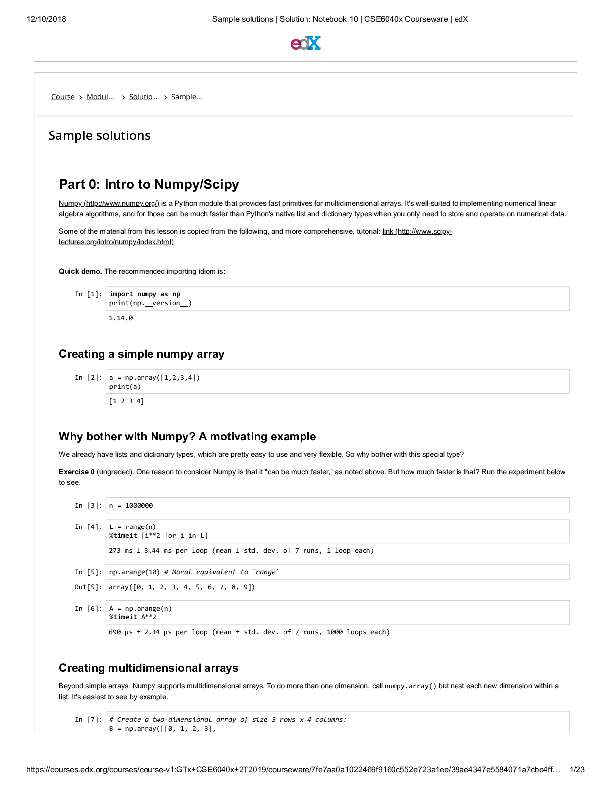
Sample solutions _ Solution_ Notebook 10 _ CSE6040x Courseware _ edX
Document Content and Description Below
Last updated: 3 months ago
Preview 1 out of 23 pages
Instant download
Buy this Document to get the Full Access Instantly
Provided by Students Who Aced it
We Verify Document Content to Gurantee Accuracy
Reviews( 0 )
Document information
Connected school, study & course
About the document
Uploaded On
Mar 24, 2021
Number of pages
23
Written in
All

Additional information
This document has been written for:
Uploaded
Mar 24, 2021
Downloads
0
Views
87
Document Keyword Tags
Recommended For You
Get more on STUDY GUIDE »
Georgia Institute Of TechnologyCSE 6040CSE 6040 Notebook 1-5 s...
Georgia Institute Of Technology - CSE 6040XSample solutions _...

Mid-term1 Solutions. GT Learners: Practice Problems for Midter...

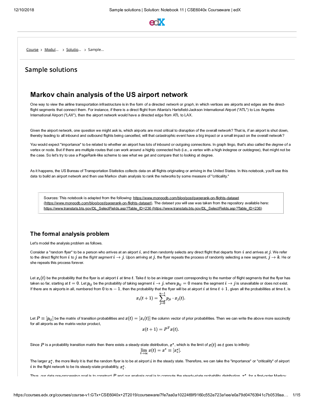
Markov chain analysis of the US airport network Michigan State...

eBook for Concepts of Programming Languages 12th Edition By R...
![Preview of eBook [PDF] Gray Hat Hacking The Ethical Hacker's Handbook 6th Edition By Allen Harper, Ry](https://browseimages.nyc3.digitaloceanspaces.com/paper-images/2025/Aug/24/lpRHB6th2025-08-24-04-5468aa70ca8c5b8.png)
eBook [PDF] Gray Hat Hacking The Ethical Hacker's Handbook 6th...
eBook 3D Printed Conducting Polymers Fundamentals, Advances, a...
![Preview of eBook [PDF] Computer Vision Challenges, Trends, and Opportunities 1st Edition By Md Atiqur](https://browseimages.nyc3.digitaloceanspaces.com/paper-images/2024/Aug/30/sO1Ff4FE2024-08-30-02-3766d1af0994f96.png)
eBook [PDF] Computer Vision Challenges, Trends, and Opportunit...
eBook Computer Vision, Challenges, Trends, and Opportunities,1...


Introduction to Programming with Java A Problem Solving Approa...
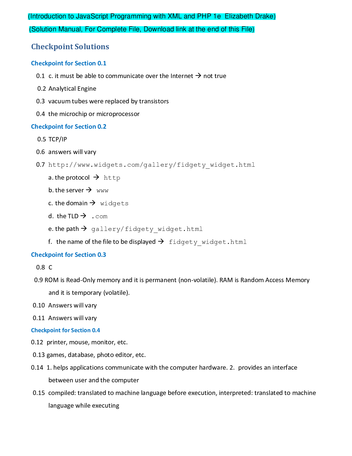
Introduction to JavaScript Programming with XML and PHP 1st Ed...
FEMA Final Exam ICS 100 (IS-100.C) Introduction to the Inciden...
Test Bank For Diversity In Organization 2nd Edition, Bell A Co...
![Preview of [eTextbook] [PDF] CompTIA Network+ Guide to Networks 9th edition By Jill West](https://browseimages.nyc3.digitaloceanspaces.com/paper-images/2025/Jan/18/o6ppor3h2025-01-18-02-55678b96c116501.png)
[eTextbook] [PDF] CompTIA Network+ Guide to Networks 9th editi...


.png)