BUSI 201 Assignment 8 Excel 2016 Skill Review 6.2 - Liberty University answers complete solutions | BUSI201 Assignment 8 Excel 2016 Skill Review 6.2

Document Content and Description Below

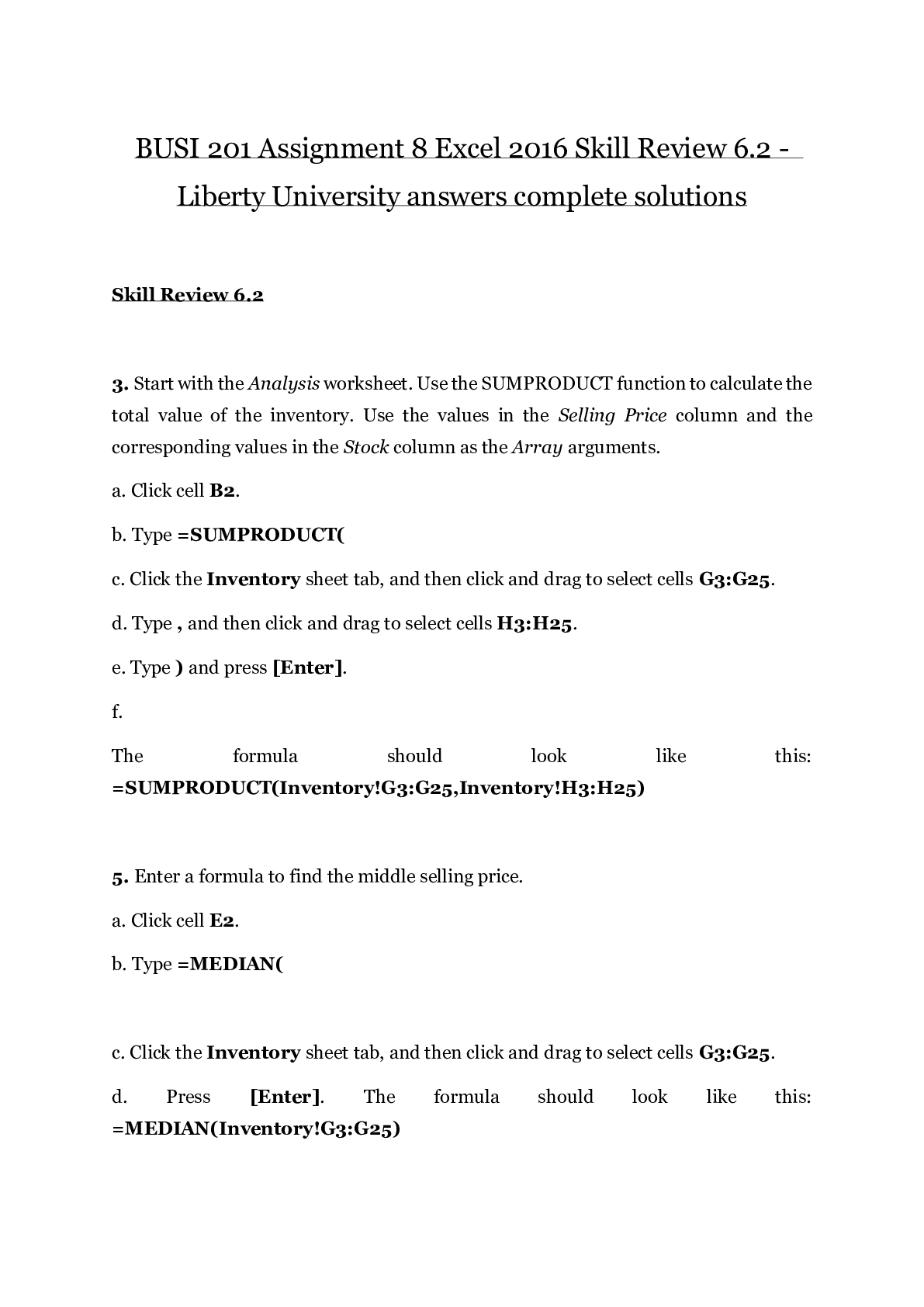
BUSI 201 Assignment 8 Excel 2016 Skill Review 6.2 - Liberty University answers complete solutions Skill Review 6.2 3. Start with the Analysis worksheet. Use the SUMPRODUCT function to calculate ... the total value of the inventory. Use the values in the Selling Price column and the corresponding values in the Stock column as the Array arguments. a. Click cell B2. b. Type =SUMPRODUCT( c. Click the Inventory sheet tab, and then click and drag to select cells G3:G25. d. Type , and then click and drag to select cells H3:H25. e. Type ) and press [Enter]. f. The formula should look like this: =SUMPRODUCT(Inventory!G3:G25,Inventory!H3:H25) 5. Enter a formula to find the middle selling price. a. Click cell E2. b. Type =MEDIAN( c. Click the Inventory sheet tab, and then click and drag to select cells G3:G25. d. Press [Enter]. The formula should look like this: =MEDIAN(Inventory!G3:G25) 7. What if there are multiple selling prices that are the most common? Enter an array formula in cells G2:G5 to find up to four most common selling prices. a. Select cells G2:G5. b. Type =MODE.MULT( c. Click the Inventory sheet tab, and then click and drag to select cells G3:G25. d. Press [Ctrl]+[Shift]+[Enter]. The formula should look like this: {=MODE.MULT(Inventory!G3:G25)} 9. Use the AVERAGEIFS function to find the average selling price of blue shoes in inventory. Use the values in the Selling Price column as the Average_range argument. Use the values in the Item Description column as theCriteria_range1 argument and use the criteria *shoes to find all items that end in the word shoes. Use the values in the Color column as the Criteria_range2 argument and use the criteria blue. a. Click cell B4. b. On the Formulas tab, in the Function Library group, click the More Functions button, point to Statistical, and select AVERAGEIFS. c. In the Function Arguments dialog, verify that the cursor is in the Average_range argument box. Click the Inventory sheet tab, and click and drag to select cells G3:G25. d. In the Function Arguments dialog, press [Tab] to move to the Criteria_range1 argument box. e. Click the Inventory sheet tab, and click and drag to select cells A3:A25. f. In the Function Arguments dialog, press [Tab] to move to the Criteria1 argument box. g. Type "*shoes"to find any text string that ends with the word shoes. h. Press [Tab]. Verify that the cursor is in the Criteria_range2 argument box. i. Click the Inventory sheet tab, and click and drag to select cells C3:C25. j. In the Function Arguments dialog, press [Tab] to move to the Criteria2 argument box. k. Type: "blue" l. Click OK. m. The formula should look like this: =AVERAGEIFS(Inventory!G3:G25,Inventory!A3:A25,"*shoes",Inventory!C3:C25,"blue") 11. Now use database functions to analyze inventory data. This method gives you more flexibility in your analysis. Once you set up the formulas, you can change the criteria in the worksheet without changing the formulas. The InventoryDB named range has been created for you to use as the Database argument. It references A2:H25 on the Inventory worksheet. Notice this named range includes the label row. Use the DAVERAGE database function to calculate the average selling price for all items with the word football in the item description. Use the wildcard character * before and after the word football to find all item descriptions with football anywhere in the text. Use the column label Selling Price as the Field argument. Remember to enclose the column label in quotation marks. Set up the criteria range. a. In cell D8, type: Item Description b. In cell D9, type: *Football* c. Click cell B9 where you will enter the formula. d. On the Formulas tab, in the Function Library group, click the Insert Function button. e. If necessary, expand the Or select a category list, and select Database. f. Double-click DAVERAGE to open the Function Arguments dialog. g. In the Database argument box, type the range name: InventoryDB h. In the Field argument box, type the column label: "Selling Price" i. Click in the Criteria argument box and then click and drag to select cells D8:D9. j. Click OK. k. The formula should look like this: =DAVERAGE(InventoryDB,"Selling Price",D8:D9) 13. Now use MATCH and INDEX to look up the item description, quantity in stock, and selling price of an item based on the inventory number. The Inventory named range has been created for you to use in these formulas. It references A3:H25 on the Inventory worksheet. Notice this named range does not include the label row. First, use MATCH to find the row position for the item listed in cell B15. Remember, the Lookup_array argument must be a single column. Require an exact match. Use absolute references so you can copy the formula. a. Click cell B16. b. On the Formulas tab, in the Function Library group, click the Lookup & Reference button, and select MATCH. c. Use an absolute reference to cell B15 for the Lookup_value argument. Type: $B$15and then press [Tab]. d. Verify that the cursor is in the Lookup_array argument box. Click the Inventory sheet tab and click and drag to select cells B3:B25. Edit the cell references to be absolute. e. In the Match_type argument box, type: 0 f. Click OK. g. The formula should look like this: =MATCH($B$15,Inventory!$B$3:$B$25,0) - - - - - - - - - - - - - - - - - - - - - - - - - - - - - - - - - - - - - - 31. In cell J4, enter the formula to calculate depreciation for year 1 using the declining balance method. a. On the Formulas tab, in the Function Library group, click the Financial button, and then select DB. b. Enter the Cost argument as an absolute cell reference so the reference will not update when you copy the formula: $G$3 c. Enter the Salvage argument as an absolute cell reference so the reference will not update when you copy the formula: $G$5 d. Enter the Life argument as an absolute cell reference so the reference will not update when you copy the formula: $G$4 e. Enter the Period argument as a relative cell reference, so the reference will update when you copy the formula: I4 f. The equipment will be in use for 12 months during the first year, so you can skip the Month argument. g. Click OK. The formula in cell J4 should look like this: =DB($G$3,$G$5,$G$4,I4) h. Copy the formula to J5:J13. 4. Enter a formula to calculate the average selling price. a. Click cell D2. b. Type =AVERAGE( c. Click the Inventory sheet tab, and then click and drag to select cells G3:G25. d. Press [Enter]. The formula should look like this: =AVERAGE(Inventory!G3:G25) 32. In cell K4, enter the formula to calculate depreciation for year 1 using the straight-line method. a. On the Formulas tab, in the Function Library group, click the Financial button, and then select SLN. b. Enter the Cost argument as an absolute cell reference so the reference will not update when you copy the formula: $G$3 c. Enter the Salvage argument as an absolute cell reference so the reference will not update when you copy the formula: $G$5 d. Enter the Life argument as an absolute cell reference so the reference will not update when you copy the formula: $G$4 e. Click OK. The formula in cell K4 should look like this: =SLN($G$3,$G$5,$G$4) f. Copy the formula to K5:K13. Notice that the straight-line method returns the same depreciation value for each period in the schedule. 33. Save and close the workbook. 34. Upload and save your project file. 35. Submit project for grading. 1. Open the start file EX2016-SkillReview-6-2. The file will be renamed automatically to include your name. 2. If the workbook opens in Protected View, click the Enable Editing button in the Message Bar at the top of the workbook so you can modify the workbook. 19. If necessary, apply the Accounting Number Format to cell B18. 20. Enter a formula using RANK.EQ to calculate the ranking of this item’s price. a. Click cell B19. b. On the Formulas tab, in the Function Library group, click the More Functions button, point to Statistical, and select RANK.EQ. c. In the Number argument box, type: 1.15and then press [Tab]. d. Verify that the cursor is in the Ref argument box. Click the Inventory sheet tab and click and drag to select cells F3:F25. e. Click OK. f. Save the file. [Show More]

Last updated: 3 years ago

Preview 1 out of 15 pages