Business > EXAM > BUSI 201 Assignment 13 Excel 2016 Skill Review 5.2 - Liberty University | BUSI201 Assignment 13 Exce (All)
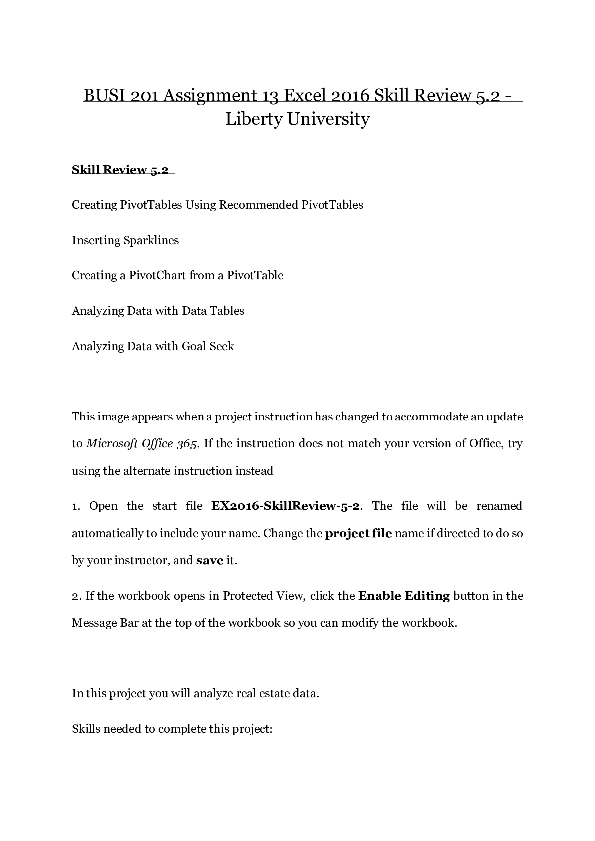
BUSI 201 Assignment 13 Excel 2016 Skill Review 5.2 - Liberty University | BUSI201 Assignment 13 Excel 2016 Skill Review 5.2
Document Content and Description Below
Last updated: 3 years ago
Preview 1 out of 9 pages
Instant download
Buy this Document to get the Full Access Instantly
Provided by Students Who Aced it
We Verify Document Content to Gurantee Accuracy
Reviews( 0 )
Document information
Connected school, study & course
About the document
Uploaded On
Jul 14, 2020
Number of pages
9
Written in
All

Additional information
This document has been written for:
Uploaded
Jul 14, 2020
Downloads
0
Views
265
Topic Tags
Recommended For You
Get more on EXAM »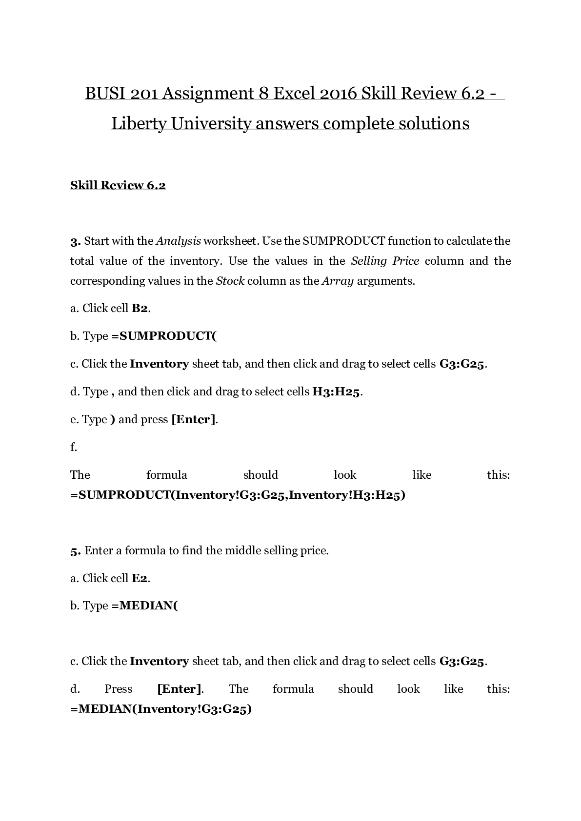
BUSI 201 Assignment 8 Excel 2016 Skill Review 6.2 - Liberty Un...

BUSI 201 Assignment 5 Excel 2016 Skill Review 3.2 - Liberty Un...

BUSI 201 Assignment 10 Excel 2016 Skill Review 7.1 Liberty Uni...
BUSI 201 Assignment 10 Excel 2016 Skill Review 7.1 answers com...
BUSI 201 Assignment 10 Excel 2016 Skill Review 7.1 Liberty Uni...
BUSI 201 Assignment 10 Excel 2016 Skill Review 7.1 Liberty Uni...
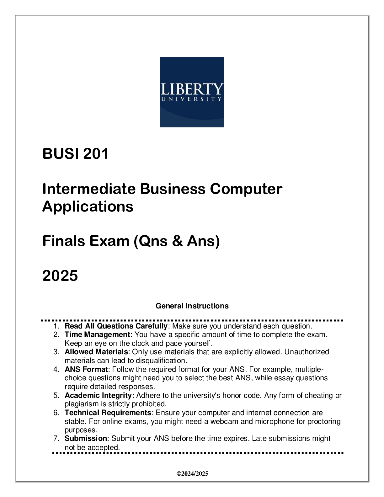
BUSI 201 Intermediate Business Computer Applications Finals Ex...
.png)
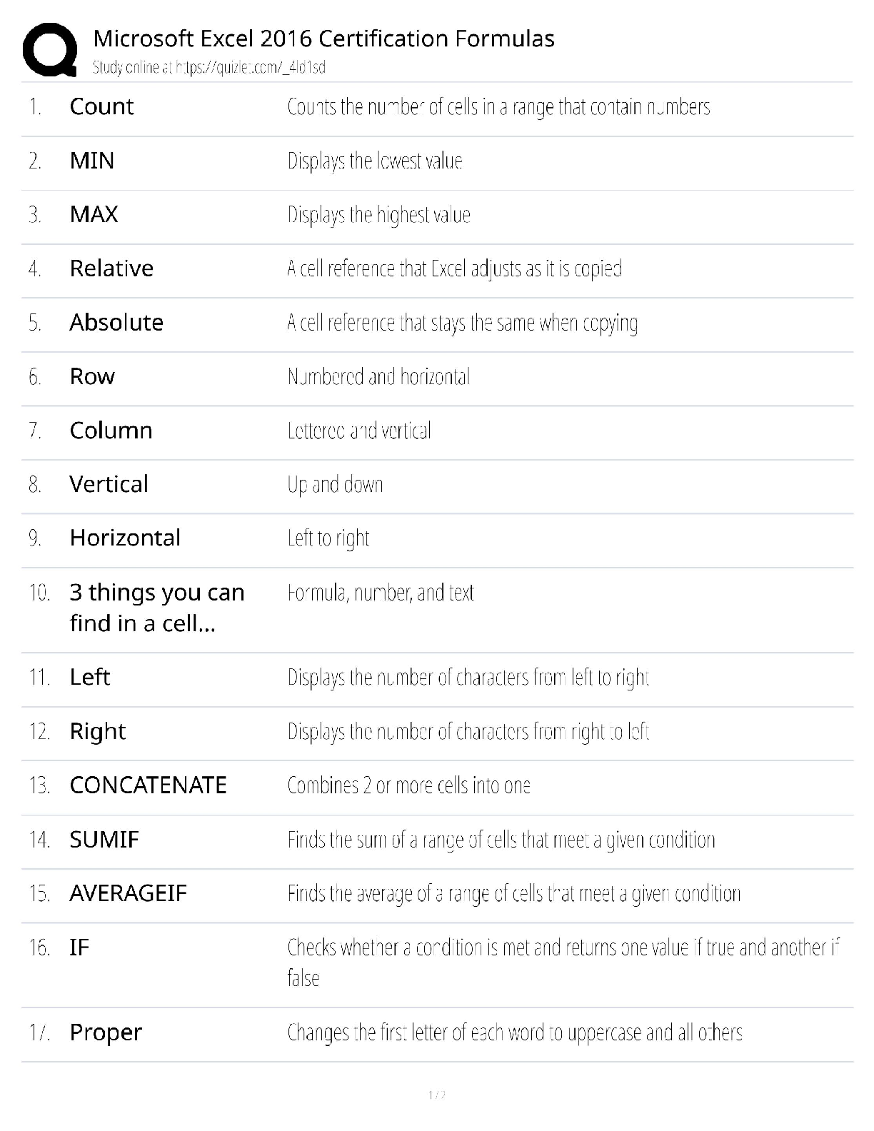
Microsoft Excel 2016 Certification / Formulas Test Bank & Stud...

Illustrated Microsoft® Office 365 & Excel 2016, Comprehensive,...

Exploring Microsoft Office Excel 2016 Comprehensive, 1e Mary A...
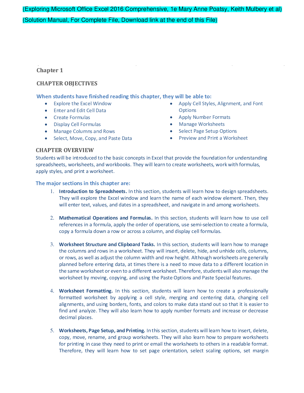
Exploring Microsoft Office Excel 2016 Comprehensive, 1e Mary A...
![Preview of [eBook] [PDF] Shelly Cashman Series Microsoft Office 365 & Excel 2016 Comprehensive, 1st E](https://browseimages.nyc3.digitaloceanspaces.com/paper-images/2023/Sep/15/L5BjICa52023-09-15-02-06650391e284334.png)
[eBook] [PDF] Shelly Cashman Series Microsoft Office 365 & Exc...
![Preview of [eBook][PDF] Exploring Microsoft Excel 2016, Comprehensive, By Mary Anne Poatsy, Mulbery,](https://browseimages.nyc3.digitaloceanspaces.com/paper-images/2023/Aug/14/n1BjMUAN2023-08-13-11-2764d93cce2341a.png)
[eBook][PDF] Exploring Microsoft Excel 2016, Comprehensive, By...
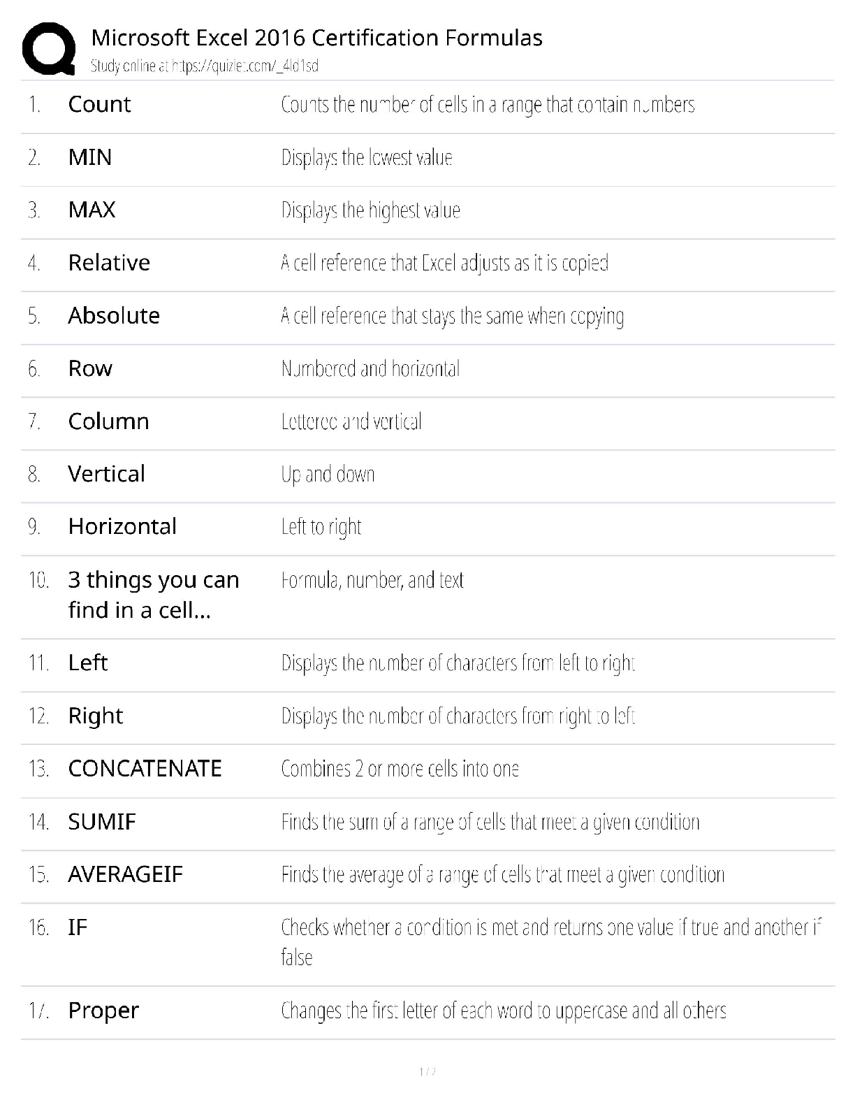
Microsoft Excel 2016 Certification Formulas / MOS Exam Prep /...


Wong's Essentials of Pediatric Nursing 11th Edition by Marilyn...
![Preview of eBook [PDF] Making Sense of Echocardiography 3rd Edition By Andrew R Houghton](https://browseimages.nyc3.digitaloceanspaces.com/paper-images/2024/Aug/31/xZQ7A7D72024-08-31-10-3566d2c7ca00d4b.png)
eBook [PDF] Making Sense of Echocardiography 3rd Edition By An...
.png)

 – Chamberlain College of Nursing.png)
 – Chamberlain College of Nursing.png)