Case Study 1 – Three Jays Corporation 831512392
Case Study Report 1: THREE JAYS CORPORATION
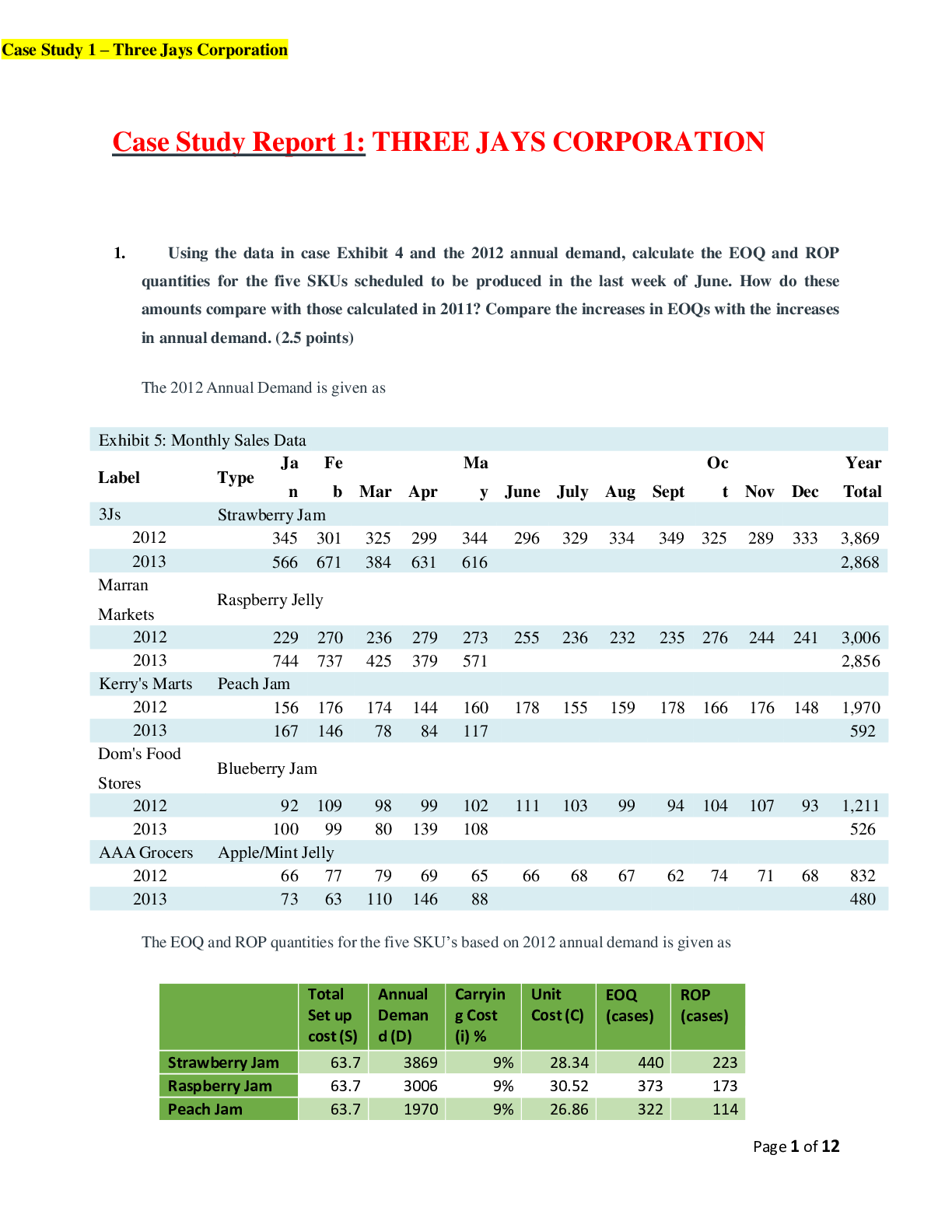
1. Using the data in case Exhibit 4 and the 2012 annual demand, calculate the EOQ and ROP
quantities for the five SKUs sc
...
Case Study 1 – Three Jays Corporation 831512392
Case Study Report 1: THREE JAYS CORPORATION
1. Using the data in case Exhibit 4 and the 2012 annual demand, calculate the EOQ and ROP
quantities for the five SKUs scheduled to be produced in the last week of June. How do these
amounts compare with those calculated in 2011? Compare the increases in EOQs with the increases
in annual demand. (2.5 points)
The 2012 Annual Demand is given as
Exhibit 5: Monthly Sales Data
Label Type
Ja
n
Fe
b Mar Apr
Ma
y June July Aug Sept
Oc
t Nov Dec
Year
Total
3Js Strawberry Jam
2012 345 301 325 299 344 296 329 334 349 325 289 333 3,869
2013 566 671 384 631 616 2,868
Marran
Markets
Raspberry Jelly
2012 229 270 236 279 273 255 236 232 235 276 244 241 3,006
2013 744 737 425 379 571 2,856
Kerry's Marts Peach Jam
2012 156 176 174 144 160 178 155 159 178 166 176 148 1,970
2013 167 146 78 84 117 592
Dom's Food
Stores
Blueberry Jam
2012 92 109 98 99 102 111 103 99 94 104 107 93 1,211
2013 100 99 80 139 108 526
AAA Grocers Apple/Mint Jelly
2012 66 77 79 69 65 66 68 67 62 74 71 68 832
2013 73 63 110 146 88 480
The EOQ and ROP quantities for the five SKU’s based on 2012 annual demand is given as
Total
Set up
cost (S)
Annual
Deman
d (D)
Carryin
g Cost
(i) %
Unit
Cost (C)
EOQ
(cases)
ROP
(cases)
Strawberry Jam 63.7 3869 9% 28.34 440 223
Raspberry Jam 63.7 3006 9% 30.52 373 173
Peach Jam 63.7 1970 9% 26.86 322 114
Page 1 of 12
Case Study 1 – Three Jays Corporation 831512392
Blueberry Jam 63.7 1211 9% 29.01 243 70
Apple/Mint Jelly 63.7 832 9% 26.32 212 48
As Demand increased from 2011 to 2012, the EOQ’s also increased
Deman
d (2010)
Deman
d (2012)
Increase
in
Demand
EOQ
(2010)
EOQ
(2012)
Increase
in EOQ
2993 3869 29.27% 387 440 13.70%
2335 3006 28.74% 329 373 13.37%
1492 1970 32.04% 280 322 15.00%
886 1211 36.68% 208 243 16.83%
625 832 33.12% 183 212 15.85%
So, if Annual Demand doubles, the EOQ will increase by sqrt(2)
2. Brodie is uncertain if the costs presented in case Exhibit 2 are appropriate for determining the
EOQs. What changes would you recommend, and why? Should the cost of the three idle part-time
workers be included when the production line is down? Using the 2012 annual demand, and your
recommendations, recalculate the EOQs for the five SKUs. (2.5 points)
In set up costs, the cost of part time workers should also be included, as they are idle at that time.
Assuming the salary of each part time worker to be half that of full time worker
So, Total salary of 3 part time workers, during idle time of 1 hour = 3*0.5*23.5 = $35.25
So, new set up cost = $63.7 + $35.25 = $98.95
In carrying cost, storage cost was considered as 0%, which should be more because, there is always an
opportunity cost of storing one inventory over another.
So, considering storage cost as 2%, new carrying cost = 6% + 2% + 3% = 11%
Some of the basic assumptions of EOQ are debated
• The demand is not uniform throughout the year, which may lead to stock outs
• The order of new batch takes time and is not done instantly. For this case, the ROP should be adjusted
to include the lead time to place order
Page 2 of 12
Case Study 1 – Three Jays Corporation 831512392
Total Set
up cost
(S)
Annual
Demand (D)
Carrying
Cost (i) %
Unit
Cost
(C)
EOQ
(cases)
ROP
(cases)
Strawberry Jam 98.95 3869 11% 28.34 496 223
Raspberry Jam 98.95 3006 11% 30.52 421 173
Peach Jam 98.95 1970 11% 26.86 363 114
Blueberry Jam 98.95 1211 11% 29.01 274 70
Apple/Mint Jelly 98.95 832 11% 26.32 238 48
Brodie’s first assignment in his internship is to update the EOQ and ROP quantities for all 141
SKUs, to reflect the current levels of demand (D), because the original calculations were done in
2011 with sales figures from 2010. This task is simple for the ROP, where:
3wks (leadtime) (annual demand)
52(wks/year)
ROP D
Making changes to the EOQ amounts is more complicated, as several logical errors exist in the
data that are used as inputs for the EOQ formula. Specifically, these are the setup cost (S), the
unit cost (C), and the inventory carrying cost, which is expressed here as a percentage (i). (Note:
Sometimes the variables i and C are combined in the EOQ formula. When this occurs, the
product of i * C is represented by the symbol H, which is the inventory holding cost in dollars
per unit, per year.)
Errors in Calculating EOQs
Setup cost (S) errors
These errors result from incorrectly including an allocation of fixed annual expenses as
components of the total setup cost. Setup costs should include only actual, out-of-pocket costs
(as should all the costs used in the calculation of the EOQ) that are directly related to setting up
the production line to make a specific item (SKU). Jake Evans and Josh Francis — as well as the
buyers who purchase the raw ingredients and packaging material for 3Js — are full-time workers
who earn a predetermined yearly salary. Consequently, reasonable changes in the number of
setups per year will not change the total cost of these individuals. Thus, regardless of whether
Page 3 of 12
Case Study 1 – Three Jays Corporation 831512392
they are employed by Fremont Jams and Jellies, or 3Js, there are no incremental costs that are
incurred with respect to setups. Therefore, the costs of changing the rails on the assembly line to
accommodate different jar sizes — as well as the costs of cleaning the equipment and switching
out the jar labels between batch sizes — should not be included in the setup cost (S). Similarly,
the costs of the two individuals employed in the kitchen should not be included in the setup
costs. These costs should be considered only as the maximum capacity f these individuals is
approached and additional people and/or equipment are required. At that point, changes could be
considered that would postpone the need for expansion, which would suggest that an appropriate
tradeoff analysis should be conducted. Thus, with the current production system, the only
relevant setup costs are the part-time wages paid to the three temporary workers, who are idle
while the line is shut down for cleaning and label changes. The setup costs are therefore equal to:
S = 3 workers * $12.50 per hour * 1 hour = $37.50
Notably, the cost of these temporary workers is not included in the original cost calculations,
most likely because they were not working and hence were not considered as part of the setup
costs. Nevertheless, their cost is an out-of-pocket expense that must be included.
Carrying cost (i) errors
The cost of carrying inventory typically consists of three components: (a) the cost of storing the
inventory, which can include storage costs (building costs, etc.) and labor and equipment costs
associated with storage, insurance, and taxes; (b) the cost of obsolescence, spoilage, and
shrinkage; and (c) the cost of capital, which is the cost of the money that is tied up in inventory.
Because FJ&J is not charging 3Js for storing its finished goods, the primary component of this
parameter is the cost of capital, which can vary. There are three scenarios:
1) If a firm has an excess of cash, then the cost of the capital tied up in inventory is the
interest lost that could have been earned by investing the money.
2) If the funds could be better used — other than in inventories — by investing in a project
that would generate additional revenues and profits, or significantly reduce costs, then
the cost of capital is the opportunity cost associated with not having the funds available
for that specific project.
Page 4 of 12
Case Study 1 – Three Jays Corporation 831512392
3) If the firm needs to borrow money to establish these inventories, then the cost of capital
is equal to the interest rate on the borrowed funds.
Here, although the cost of borrowing capital is 6%, the actual cost of capital is the opportunity
cost associated with the inability of the firm to launch a new marketing campaign due to its lack
of funds, which is estimated to be 20%. This is the projected contribution to overhead and profit
that the additional revenues would generate. The 3% that is used for storage recognizes that FJ&J
is not charging for the actual storage of finished goods, but it does include the cost of
obsolescence, insurance, and taxes. Thus, the cost of carrying inventory is:
i = 20% + 3% = 23%
Unit cost errors (C)
Again, we should include only costs that represent out-of-pocket costs associated with the jams
and jellies that are being produced. The components of the unit cost (C) should therefore include
only those costs that are directly incurred each time a run is made. This is represented in case
Exhibit 3 as the “Total Variable Cost,” which does not include the fixed overhead cost allocation;
that allocation is currently included in the calculations.
Assumptions in the EOQ Calculations
There are several assumptions inherent in the EOQ formula, many of which are not applicable to
the 3Js situation. These include:
1) Unit cost remains constant and does not vary (as would be the case with quantity disc
unts). This is valid, given the information in the case.
2) There are no stock-out costs. While these costs are not mentioned in the case, they need
to be considered in determining how much inventory in the form of safety stock to have
on hand.
3) Demand is constant and known. At 3Js, however, the firm is g owing; the actual demand
is not known, but estimated based on some type of forecasting method.
4) Production capacity is always available when it is needed. In other words, there is no lag
time between when product is required and when it is produced. At 3Js, however, the
production of a specific size jar is scheduled for a given week, and any requirements
Page 5 of 12
Case Study 1 – Three Jays Corporation 831512392
prior to that week will be delayed until that time. (Note: When Assumptions 3 and 4 are
valid, stock-outs most likely will not occur, which is why there is no need to consider
them in the EOQ formula.)
5) There are no interactions among the different items produced. There are significant
interactions at 3Js, however, because of the relatively high setup cost associated with
changing the jar size. As a result, items are grouped to reduce this cost, thereby affecting
when they are produced.
Comparing Old and New EOQs
The calculation of the original EOQs shown in Table 1 below (and the attached Excel
spreadsheet) are presented in case Exhibit 4:
Table 1. EOQ Calculations Using Existing Method (see case Exhibit 2) and 2010 Sales Data
Product (12 oz.) 3Js Marran Kerry Dom AAA
sales/wk 58 45 29 17 12
S = Setup Cost 63.70 63.70 63.70 63.70 63.70
D = Annual Demand (cases) 2,993 2,335 1,492 886 625
I = Carry Cost 9% 9% 9% 9% 9%
C = Full Cost/Case 28.34 30.52 26.86 29.01 26.32
EOQ (old) 387 329 280 208 183
ROP (3 weeks) 172.7 134.7 86.1 51.1 36.1
If we just update this using the 2012 sales data, we have the comparison shown in Table 2 below
(and the attached Excel spreadsheet):
Table 2. EOQ Calculations Using Existing Method (see case Exhibit 2) and 2012 Sales Data
Product (12 oz.) 3Js Marran Kerry Dom AAA
sales/wk 74 58 38 23 16
S = Setup Cost 63.70 63.70 63.70 63.70 63.70
D = Annual Demand (cases) 3,869 3,006 1,970 1,211 832
I = Carry Cost 9% 9% 9% 9% 9%
C = Full Cost/Case 28.34 30.52 26.86 29.01 26.32
EOQ (old) 440 373 322 243 212
Page 6 of 12
Case Study 1 – Three Jays Corporation 831512392
% Increase - Sales 29.3% 28.7% 32.0% 36.7% 33.1%
% Increase - EOQ 13.7% 13.5% 14.9% 16.9% 15.4%
The increases in sales range from 28.7% to 36.7%, but the increase in EOQs ranges from 13.5%
to 16.9%. This difference is attributable
[Show More]


.png)