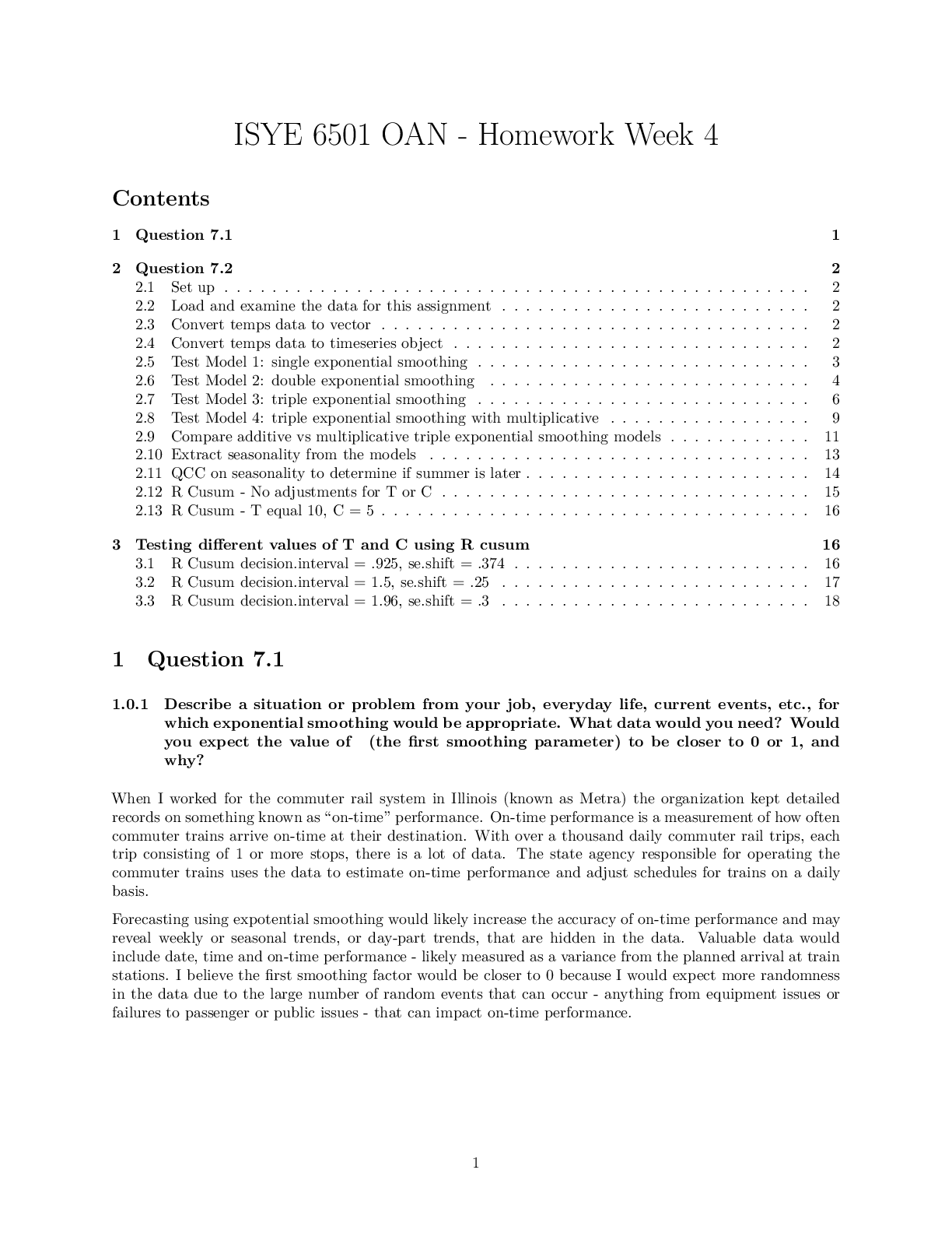
ISYE 6501 OAN - Homework Week 4 Latest Update

ISYE 6501 OAN - Homework Week 4 Contents 1 Question 7.1 1 2 Question 7.2 2 2.1 Set up . . . . . . . . . . . . . . . . . . . . . . . . . . . . . . . . . . . . . . . . . . . . . . . . . 2 2.2 Load and examine the data ...

ISYE 6501 OAN - Homework Week 4 Contents 1 Question 7.1 1 2 Question 7.2 2 2.1 Set up . . . . . . . . . . . . . . . . . . . . . . . . . . . . . . . . . . . . . . . . . . . . . . . . . 2 2.2 Load and examine the data for this assignment . . . . . . . . . . . . . . . . . . . . . . . . . . 2 2.3 Convert temps data to vector . . . . . . . . . . . . . . . . . . . . . . . . . . . . . . . . . . . . 2 2.4 Convert temps data to timeseries object . . . . . . . . . . . . . . . . . . . . . . . . . . . . . . 2 2.5 Test Model 1: single exponential smoothing . . . . . . . . . . . . . . . . . . . . . . . . . . . . 3 2.6 Test Model 2: double exponential smoothing . . . . . . . . . . . . . . . . . . . . . . . . . . . 4 2.7 Test Model 3: triple exponential smoothing . . . . . . . . . . . . . . . . . . . . . . . . . . . . 6 2.8 Test Model 4: triple exponential smoothing with multiplicative . . . . . . . . . . . . . . . . . 9 2.9 Compare additive vs multiplicative triple exponential smoothing models . . . . . . . . . . . . 11 2.10 Extract seasonality from the models . . . . . . . . . . . . . . . . . . . . . . . . . . . . . . . . 13 2.11 QCC on seasonality to determine if summer is later . . . . . . . . . . . . . . . . . . . . . . . . 14 2.12 R Cusum - No adjustments for T or C . . . . . . . . . . . . . . . . . . . . . . . . . . . . . . . 15 2.13 R Cusum - T equal 10, C = 5 . . . . . . . . . . . . . . . . . . . . . . . . . . . . . . . . . . . . 16 3 Testing different values of T and C using R cusum 16 3.1 R Cusum decision.interval = .925, se.shift = .374 . . . . . . . . . . . . . . . . . . . . . . . . . 16 3.2 R Cusum decision.interval = 1.5, se.shift = .25 . . . . . . . . . . . . . . . . . . . . . . . . . . 17 3.3 R Cusum decision.interval = 1.96, se.shift = .3 . . . . . . . . . . . . . . . . . . . . . . . . . . 18 1 Question 7.1 1.0.1 Describe a situation or problem from your job, everyday life, current events, etc., for which exponential smoothing would be appropriate. What data would you need? Would you expect the value of ff (the first smoothing parameter) to be closer to 0 or 1, and why? When I worked for the commuter rail system in Illinois (known as Metra) the organization kept detailed records on something known as “on-time” performance. On-time performance is a measurement of how often commuter trains arrive on-time at their destination. With over a thousand daily commuter rail trips, each trip consisting of 1 or more stops, there is a lot of data. The state agency responsible for operating the commuter trains uses the data to estimate on-time performance and adjust schedules for trains on a daily basis. Forecasting using expotential smoothing would likely increase the accuracy of on-time performance and may reveal weekly or seasonal trends, or day-part trends, that are hidden in the data. Valuable data would include date, time and on-time performance - likely measured as a variance from the planned arrival at train stations. I believe the first smoothing factor would be closer to 0 because I would expect more randomness in the data due to the large number of random events that can occur - anything from equipment issues or failures to passenger or public issues - that can impact on-time performance. 1 2 Question 7.2 2.0.1 Using the 20 years of daily high temperature data for Atlanta (July through October) from Question 6.2 (file temps.txt), build and use an exponential smoothing model to help make a judgment of whether the unofficial end of summer has gotten later over the 20 years. (Part of the point of this assignment is for you to think about how you might use exponential smoothing to answer this question. Feel free to combine it with other models if you’d like to. There’s certainly more than one reasonable approach.) 2.0.2 Note: in R, you can use either HoltWinters (simpler to use) or the smooth package’s es function (harder to use, but more general). If you use es, the Holt-Winters model uses model=”AAM” in the function call (the first and second constants are used “A”dditively, and the third (seasonality) is used “M”ultiplicatively; the documentation doesn’t make that clear). 2.1 Set up # Clear the enviroment rm(list = ls()) # Set a working directory for this particular project setwd("~/OneDrive/GATechMS/ISYE6501/Week4") # Set a seed in case we work with any random number generators set.seed(52) # Load the libraries we need for this analysis library(qcc) ## Package 'qcc' version 2.7 ## Type 'citation("qcc")' for citing this R package in publications. 2.2 Load and examine the data for this assignment # Load the data from the file, name is uscrime.data temps.data <- read.table("temps.txt", header = TRUE, stringsAsFactors = FALSE) 2.3 Convert temps data to vector #Convert to vector data, vector.temps.data<-as.vector(unlist(temps.data[2:21])) 2.4 Convert temps data to timeseries object #convert to time series ts.vector.temps.data<-ts(vector.temps.data, start=1996, frequency = 123)