ISYE - 6501 Homework 2
Due Date: Thursday, September 3rd, 2020
Contents
1 ISYE - 6501 Homework 2 2
2 Homework Analysis 2
2.1 Analysis 3.1 . . . . . . . . . . . . . . . . . . . . . . . . . . . . . . . . . . . . . . .
...
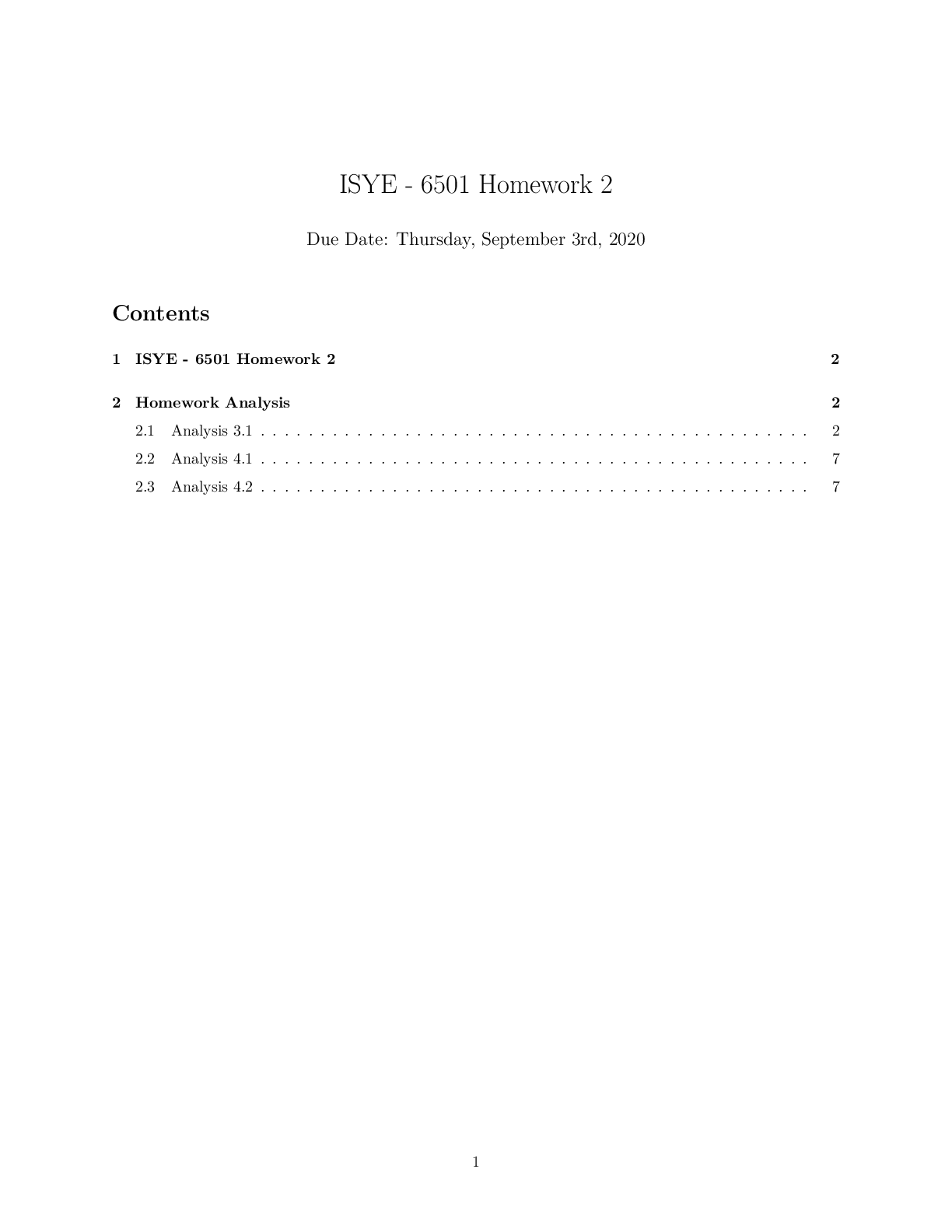
ISYE - 6501 Homework 2
Due Date: Thursday, September 3rd, 2020
Contents
1 ISYE - 6501 Homework 2 2
2 Homework Analysis 2
2.1 Analysis 3.1 . . . . . . . . . . . . . . . . . . . . . . . . . . . . . . . . . . . . . . . . . . . . . . 2
2.2 Analysis 4.1 . . . . . . . . . . . . . . . . . . . . . . . . . . . . . . . . . . . . . . . . . . . . . . 7
2.3 Analysis 4.2 . . . . . . . . . . . . . . . . . . . . . . . . . . . . . . . . . . . . . . . . . . . . . . 7
11 ISYE - 6501 Homework 2
This document contains my analysis for ISYE - 6501 Homework 2 which is due on Thursday, September 3rd,
2020. Enjoy!
2 Homework Analysis
2.1 Analysis 3.1
Q: Using the same data set (credit_card_data.txt or credit_card_data-headers.txt) as in Question 2.2, use
the ksvm or kknn function to find a good classifier.
(a) using cross-validation (do this for the k-nearest-neighbors model; SVM is optional)
RESULTS
By using cross-validation at 10 folds on a k-nearest-neighbors (KNN) model, at k=15 with a rectangular
kernel, we were able to achieve an accuracy score of roughly 85% (85.47009%). This means that 85 out of
every 100 applicants is predicted correct!
THE CODE:
# needed library
rm(list=ls())
library(kknn)
library(dplyr)
set.seed(12345)
# read data into R
data_path <- "data 3.1/"
data_filename <- "credit_card_data-headers.txt"
credit_data <- read.delim(paste0(data_path, data_filename), header=TRUE)
# train-valid-test-split
sample_split <- sample(1:3, size=nrow(credit_data), prob=c(0.7,0.15,0.15),
replace = TRUE)
train_credit <- credit_data[sample_split==1,]
valid_credit <- credit_data[sample_split==2,]
test_credit <- credit_data[sample_split==3,]
# training our model
train_model <- train.kknn(R1~., train_credit, kmax=100, scale=TRUE, kcv=10,
kernel=c("rectangular", "triangular",
"epanechnikov", "gaussian",
"rank", "optimal"),
kpar=list())
train_model
##
## Call:
2## train.kknn(formula = R1 ~ ., data = train_credit, kmax = 100, kernel = c("rectangular", "triangul
##
## Type of response variable: continuous
## minimal mean absolute error: 0.221968
## Minimal mean squared error: 0.1175795
## Best kernel: rectangular
## Best k: 15
Using cross-validation at 10 folds, we can see that the best kernel for our model is rectangular with a k of
15. Now that we have the best parameters for our model, let’s use them to train our validation data.
# validating our model
valid_model <- train.kknn(R1~., valid_credit, ks=15, kernel="rectangular", scale=TRUE, kpar=list())
valid_pred <- round(predict(valid_model, valid_credit))
accuracy_score <- sum(valid_pred == valid_credit[,11]) / nrow(valid_credit)
accuracy_score * 100
## [1] 91
Our validation model provides and accuracy score of 91%. Now, let’s run the model through our test data
to measure its true performance on data it hasn’t seen with before.
# run test data through model
test_pred <- round(predict(valid_model, test_credit))
accuracy_score <- sum(test_pred == test_credit[,11]) / nrow(test_credit)
accuracy_score * 100
## [1] 85.47009
Our test data provides an accuracy score of roughly 85%. This is lower than the validation data accuracy score (91%). We can conclude that our model favored the randomness of the data it was validated
(valid_credit) on over data it hadn’t seen before (test_credit). Thus, being closer to the model’s true
performance.
(b) splitting the data into training, validation, and test data sets (pick either KNN or SVM;
the other is optional).
RESULTS
A train-valid-test split allows us to produce a Support Vector Machine (SVM) with a splinedot kernel and
C value of 1 that achieves an accuracy score of roughly 82% (82.05128).
OUR CLASSIFIER EQUATION
Based on the SVM model classifier equation below:
classifier = β0 + β1x1 + β2x2...βpxi
With an error margin (C) of 1 and the splinedot kernel, we produced the following classifier equation:
classifier = −0.1994897 + 0.040093784x1 + 0.105580560x2 − 0.023190123x3 + 0.019249666x4 +
0.379332434x5 − 0.118072986x6 − 0.001239596x7 − 0.025400298x8 + 0.026589464x9 + 0.101784342x10
3THE CODE:
# needed library
library(kernlab)
library(magicfor)
library(ggplot2)
library(hrbrthemes)
set.seed(12345)
# train-valid-test-split
sample_split <- sample(1:3, size=nrow(credit_data), prob=c(0.7,0.15,0.15),
replace = TRUE)
train_credit <- credit_data[sample_split==1,]
valid_credit <- credit_data[sample_split==2,]
test_credit <- credit_data[sample_split==3,]
# training our model
magic_for(print, silent = TRUE)
kerns <- list("rbfdot", "polydot", "vanilladot", "tanhdot", "laplacedot",
"besseldot", "anovadot", "splinedot")
for (kern in kerns) {
train_model <- ksvm(R1~., data=train_credit, type="C-svc", kernel=kern,
C=1, scaled=TRUE, kpar=list())
train_pred <- predict(train_model, train_credit[,1:10])
accuracy <- sum(train_pred == train_credit[,11]) / nrow(train_credit)
print(accuracy)
}
kern_accuracy <- magic_result_as_dataframe()
# displaying our model’s best kernel
ggplot(kern_accuracy, aes(x=kern, y=accuracy, color=accuracy)) +
geom_point(size=8) +
ylim(c(.7, 1)) +
labs(title="Accuracy Scores vs Kernel Function",
y="Accuracy Scores",
x="Kernel Function") +
theme(plot.title = element_text(hjust=0.5),
axis.title.x = element_text(hjust=0.5, size=14),
axis.title.y = element_text(hjust=0.5, size=14),
legend.position = "None",
axis.line=element_line(size = 1, linetype="solid")) +
geom_vline(xintercept="splinedot", linetype="dotted",
color="blue", size=2)
[Show More]