INTRODUCTION
When trying to decide what car to buy, the real value is not necessarily determined by how much you spend
on the initial purchase. Instead, cars that are reliable and don’t cost much to own often represent
...
INTRODUCTION
When trying to decide what car to buy, the real value is not necessarily determined by how much you spend
on the initial purchase. Instead, cars that are reliable and don’t cost much to own often represent the
best values. But, no matter how reliable or inexpensive a car may cost to own, it must also perform well.
To measure value, a consumer report developed a statistic referred to as a value score. The value score is
based upon five-year owner costs, overall road-test scores, and predicted reliability ratings. Five-year
owner costs are based on the expenses incurred in the first five years of ownership, including
depreciation, fuel, maintenance and repairs, and so on.
Using a national average of 12,000 miles per year, an average cost per mile driven is used as the
measure of five-year owner costs. Road-test scores are the results of more than 50 tests and evaluations
and are based upon a 100-point scale, with higher scores indicating better performance, comfort,
convenience, and fuel economy. The highest road-test score obtained in the tests conducted by
consumer report was a 99 for a Lexus LS 460L.
Predicted-reliability ratings (15 Poor, 25 Fair, 35 Good, 45 Very Good, and 55 Excellent) are based on
data from consumer report Annual Auto Survey.
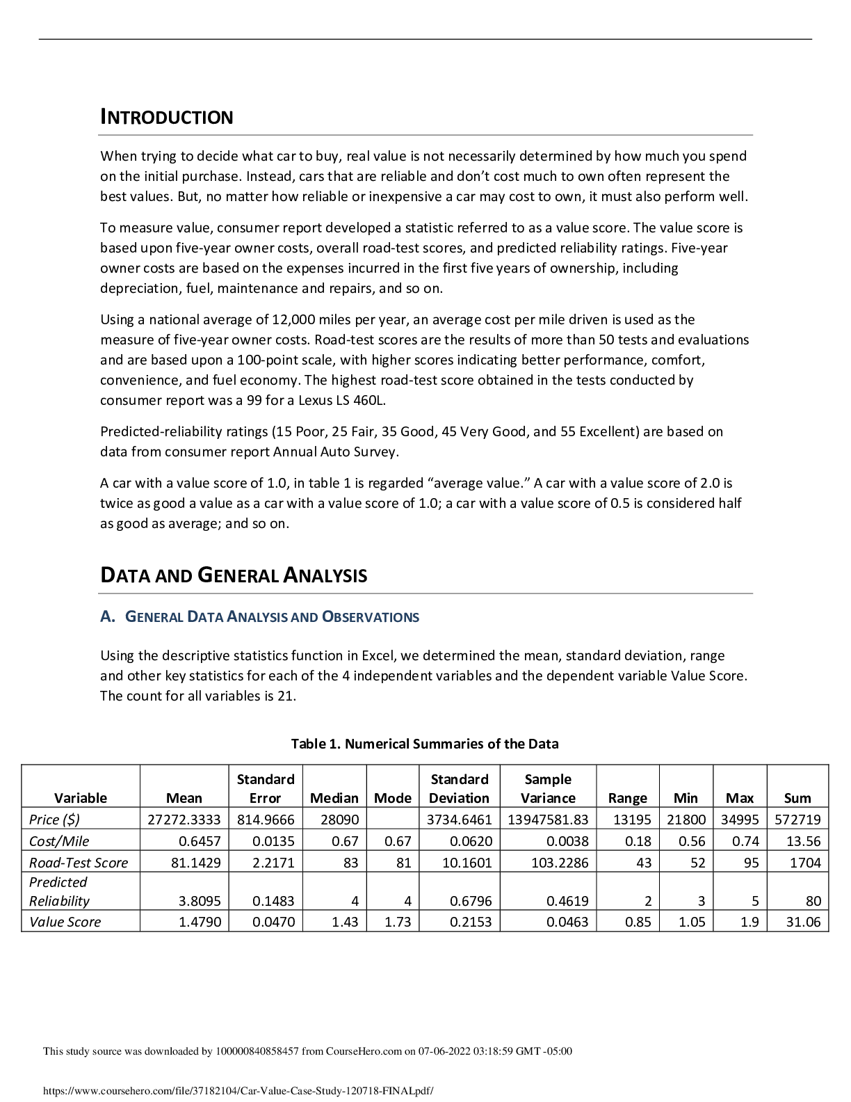
A car with a value score of 1.0, in table 1 is regarded “average value.” A car with a value score of 2.0 is
twice as good a value as a car with a value score of 1.0; a car with a value score of 0.5 is considered half
as good as average; and so on.
DATA AND GENERAL ANALYSIS
A. GENERAL DATA ANALYSIS AND OBSERVATIONS
Using the descriptive statistics function in Excel, we determined the mean, standard deviation, range
and other key statistics for each of the 4 independent variables and the dependent variable Value Score.
The count for all variables is 21.
Table 1. Numerical Summaries of the Data
Variable Mean
Standard
Error Median Mode
Standard
Deviation
Sample
Variance Range Min Max Sum
Price ($) 27272.3333 814.9666 28090 3734.6461 13947581.83 13195 21800 34995 572719
Cost/Mile 0.6457 0.0135 0.67 0.67 0.0620 0.0038 0.18 0.56 0.74 13.56
Road-Test Score 81.1429 2.2171 83 81 10.1601 103.2286 43 52 95 1704
Predicted
Reliability 3.8095 0.1483 4 4 0.6796 0.4619 2 3 5 80
Value Score 1.4790 0.0470 1.43 1.73 0.2153 0.0463 0.85 1.05 1.9 31.06
This study source was downloaded by 100000840858457 from CourseHero.com on 07-06-2022 03:18:59 GMT -05:00
https://www.coursehero.com/file/37182104/Car-Value-Case-Study-120718-FINALpdf/B. REGRESSION ANALYSES TO DEVELOP ESTIMATED REGRESSION EQUATIONS
For simple linear regression, the least squares estimates are denoted as b0 and b1. Using these
estimates, an estimated regression equation is constructed: ŷ = b0 + b1x. Before we solved for each of
the estimations, we showed the data graphically in a scatter diagram. The independent variable is
located on the x-axis and the dependent variable is located on the y-axis. We then used the regression
function in Excel to obtain the below statistical output summaries.
1. Estimated regression equation that could be used to predict the value score given the price of
the car.
ŷ = value score, b0 = 1.8538, and b1x = -1E-05x; therefore the estimated equation is:
value score = 1.8538 + -1E-05x
2. Estimated regression equation that could be used to predict the value score given the fiveyear owner costs (cost/mile).
ŷ = value score, b0 = 2.5837, and b1x = -1.7108x; therefore the estimated equation is: value
score = 2.5837 + -1.7108x
Coefficients
Standard
Error t Stat P-value
Lower
95%
Upper
95%
Lower
95.0%
Upper
95.0%
Intercept 1.8538 0.3534 5.2465 0.0000 1.1143 2.5934 1.1143 2.5934
Price ($) -1.374E-05 1.2842E-05 -1.0700969 0.2979821 -4.06214E-05 1.31E-05 -4.06214E-05 1.31E-05
This study source was downloaded by 100000840858457 from CourseHero.com on 07-06-2022 03:18:59 GMT -05:00
https://www.coursehero.com/file/37182104/Car-Value-Case-Study-120718-FINALpdf/3. Estimated regression equation that could be used to predict the value score given the roadtest score.
ŷ = value score, b0 = 2.6375, and b1x = 0.0104x; therefore the estimated equation is:
value score = 2.6375 + 0.0104x
4. Estimated regression equation that could be used to predict the value score given the
predicted reliability.
ŷ = value score, b0 = 0.9157, and b1x = 0.1479x; therefore the estimated equation is:
value score = 0.9157 + 0.1479x
Coefficients
Standard
Error t Stat P-value Lower 95%
Upper
95%
Lower
95.0%
Upper
95.0%
Intercept 2.5837 0.4494 5.7494 0.0000 1.6432 3.5243 1.6432 3.5243
Cost/Mile -1.7108 0.6929 -2.4690 0.0232 -3.1611 -0.2605 -3.1611 -0.2605
Coefficients
Standard
Error t Stat P-value
Lower
95%
Upper
95%
Lower
95.0%
Upper
95.0%
Intercept 0.6375 0.3465 1.8398 0.0815 -0.0877 1.3627 -0.0877 1.3627
Road-Test Score 0.0104 0.0042 2.4470 0.0243 0.0015 0.0192 0.0015 0.0192
USED TO PREDICT THE VALUE OF A CAR
To develop a multiple regression model, we completed the following steps:
• Used the F test to assess overall significance
• Used the t-test to assess the significance of each individual variable
• Leveraged Excel’s Regression function to develop our multiple regression model
• applied our model to the data received to assess the accuracy of our model
• Used our multiple regression model to predict a value score
1. Testing for overall significance: The F Test
The F test is used to determine whether a significant relationship exists between the
dependent variable, value score, and the set of all the independent variables. The
hypothesis is:
• H0: B1 = B2 = B3 = B4 = 0
• Ha: One or more of the parameters is not equal to zero
• The F test statistic: F = MSR/MSE
Using the regression function in Excel we determine that the p-value associated with the
F test is 1.46-07 which is < our level of significance (.05) so we can reject H0 and
conclude that a significant relationship exists between the value score and the
independent variables.
ANOVA
df SS MS F Significance F
Regression 4 0.827095965 0.206773991 33.18838602 1.45821E-07
Residual 16 0.099684988 0.006230312
Total 20 0.926780952
Coefficients
Standard
Error t Stat P-value
Lower
95%
Upper
95%
Lower
95.0%
Upper
95.0%
Intercept 0.9157 0.2485 3.6852 0.0016 0.3956 1.4357 0.3956 1.4357
Predicted Reliability 0.1479 0.0643 2.3015 0.0329 0.0134 0.2824 0.0134 0.2824
A separate t test is conducted for each of the independent variables in the model to
determine individual variable significance. In each case our hypothesis is:
• H0: Bx = 0
• Ha: Bx not equal to 0
• We can reject H0 if p-value of the test statistic t is <= our level of significance
.05
Using the regression function in excel we determine the p-value associated with the t
statistic for each independent variable. Through this analysis we can see that the pvalue associated with the t test for Price is > our level of significance .05, so we can
conclude that Price is not significant and exclude it from the multiple regression model.
We can also see that the p-value for all other variables is <= our level of significance .05
and therefore conclude that they are significant.
Coefficients
Standard
Error t Stat P-value
Intercept 0.945229969 0.293461218 3.220970648 0.005337167
Price ($) -5.09399E-06 1.0609E-05 -0.480155214 0.637615595
Cost/Mile -1.836324199 0.601194493 -3.054459451 0.007567863
Road-Test Score 0.013082378 0.001917875 6.821289908 4.10731E-06
Predicted
Reliability 0.209197204 0.028848811 7.251501744 1.9358E-06
3. Development of the multiple regression model and predicting value
Given that Price has been determined to not be significant, we can now make a decision
on whether or not to include it in our multiple regression model.
Analysis of the data using the excel regression function provides the following insights:
With price included in the model we have:
Y = .945 + (-5.09 -06 * price) + (-1.84 * cost/mile) + (.01 * road-test score) + (.21 * reliability)
Coefficients
Intercept 0.945229969
Price ($) -5.09399E-06
Cost/Mile -1.836324199
Road-Test Score 0.013082378
Predicted Reliability 0.209197204
R Square 0.892439537
Adjusted R Square 0.865549422
function we have:
Y = 1.02 + (-2.09 * cost/mile) + (.01 * road-test score) + .20 * reliability)
Coefficients
Intercept 1.020320966
Cost/Mile -2.089708136
Road-Test Score 0.012714873
Predicted Reliability 0.203794473
We note that both equations have similar coefficients of determination (R2 = .89 for
both) but the adjusted multiple coefficient of determination (Adjusted R Square) is
slightly improved for the regression model with price removed due to insignificance.
We determine that we would progress with this multiple regression model for future
predictions.
4. Using the multiple regression model to predict a value score
Using our multiple regression model, we predict the value score for the ABC-Cars-M380
model to be:
Car Price ($) Cost/Mile
Road-Test
Score
Predicted
Reliability
Predicted
Value Score
ABC-Cars-M380 32000 0.9 83 5 1.21
CONCLUSION
From our analysis, we discovered that when modeling the provided data, the variable of Price is not
significant and does not need to be included. All other variables are significant and may have an impact
on the value score.
We also see that using a regression model to predict value does provide a reliable estimate. To confirm
the validity of the model we used the multiple regression model to compare the actual values of our
dependent variable against the predicted value and achieved the following:
Car Actual
Value Score
Predicted
Value Score
Nissan Altima 2.5 S (4-cyl.) 1.75 1.76
Kia Optima LX (2.4) 1.73 1.65
R Square 0.890889665
Adjusted R Square 0.8716349
Ford Fusion Hybrid 1.70 1.79
Honda Accord LX-P (4-cyl.) 1.62 1.68
Mazda6 i Sport (4-cyl.) 1.60 1.55
Hyundai Sonata GLS (2.4) 1.58 1.59
Ford Fusion SE (4-cyl.) 1.55 1.61
Chevrolet Malibu LT (4-cyl.) 1.48 1.38
Kia Optima SX (2.0T) 1.43 1.40
Ford Fusion SEL (V6) 1.42 1.45
Nissan Altima 3.5 SR (V6) 1.42 1.58
Hyundai Sonata Limited (2.0T) 1.39 1.38
Honda Accord EX-L (V6) 1.36 1.38
Mazda6 s Grand Touring (V6) 1.34 1.32
Ford Fusion SEL (V6, AWD) 1.32 1.31
Subaru Legacy 3.6R Limited 1.29 1.27
Chevrolet Malibu LTZ (V6) 1.20 1.29
Chrysler 200 Limited (V6) 1.20 1.24
Chevrolet Impala LT (3.6) 1.05 1.03
Mercedes EC320D 1.90 1.74
[Show More]
