Mathematics > QUESTIONS & ANSWERS > MATH 3589 Calculous - Ohio State University. Introduction to Financial Mathematics Homework Assignme (All)
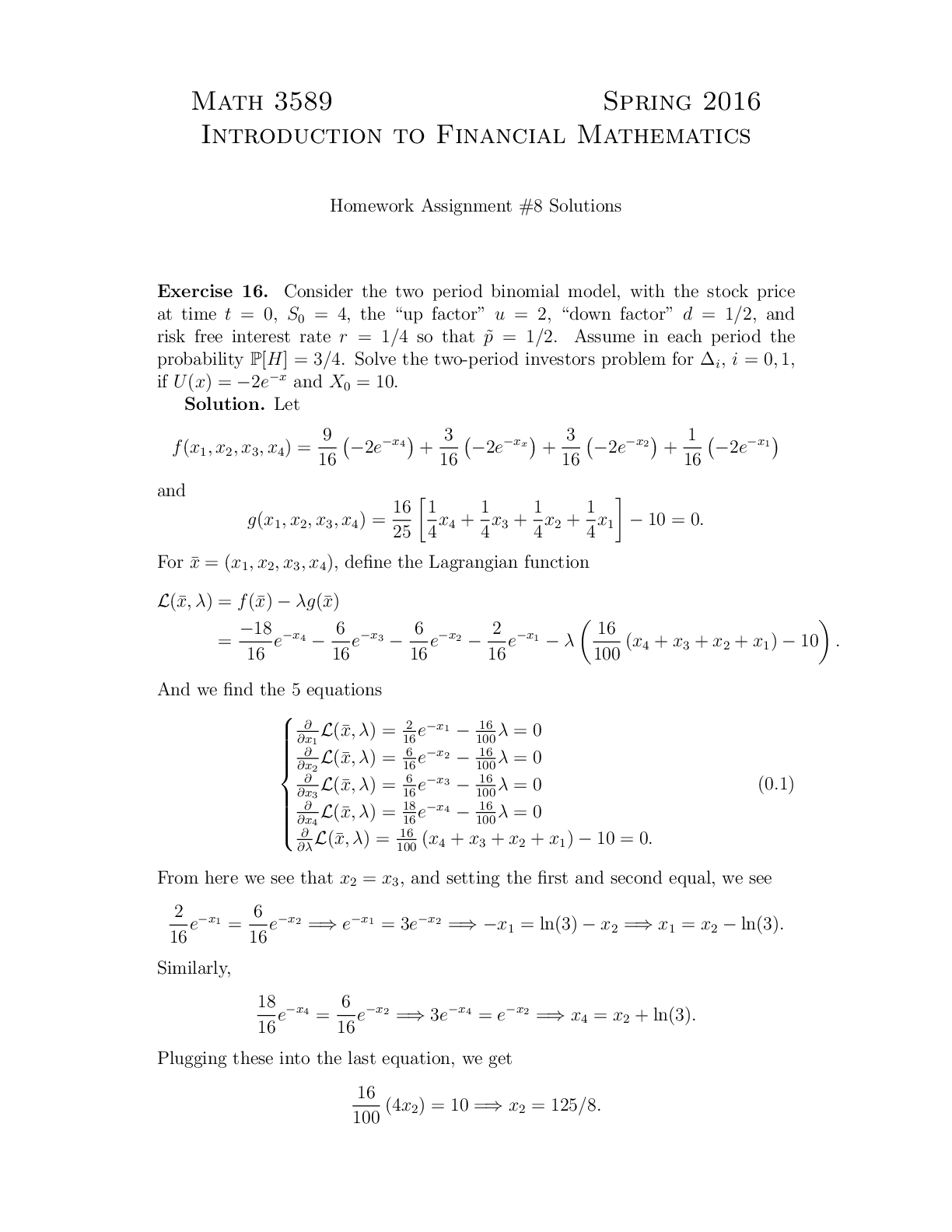
MATH 3589 Calculous - Ohio State University. Introduction to Financial Mathematics Homework Assignment #8 Solutions.
Document Content and Description Below
Last updated: 3 years ago
Preview 1 out of 5 pages
Instant download
Buy this Document to get the Full Access Instantly
Provided by Students Who Aced it
We Verify Document Content to Gurantee Accuracy
Reviews( 0 )
Document information
Connected school, study & course
About the document
Uploaded On
Apr 13, 2023
Number of pages
5
Written in
All

Additional information
This document has been written for:
Uploaded
Apr 13, 2023
Downloads
0
Views
82
Topic Tags
Recommended For You
Get more on QUESTIONS & ANSWERS »
An Introduction to Financial Mathematics Option Valuation 2nd...
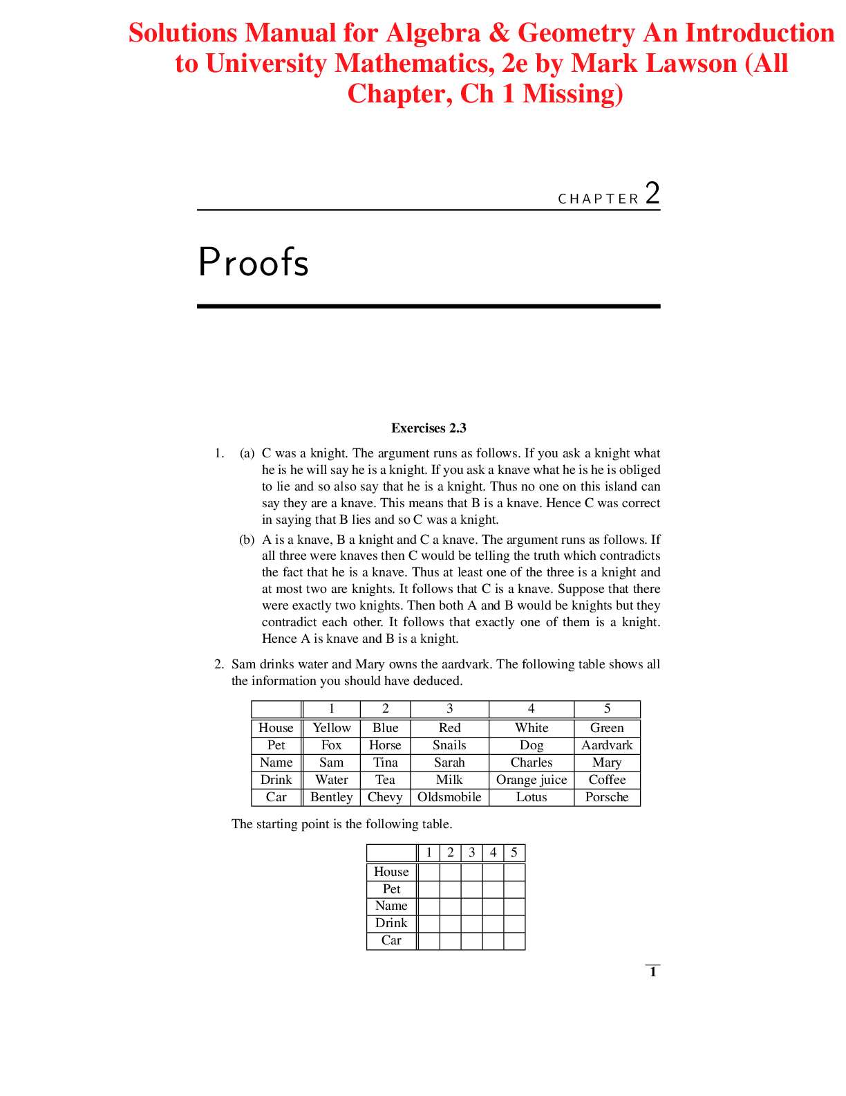
Algebra & Geometry An Introduction to University Mathematics 2...
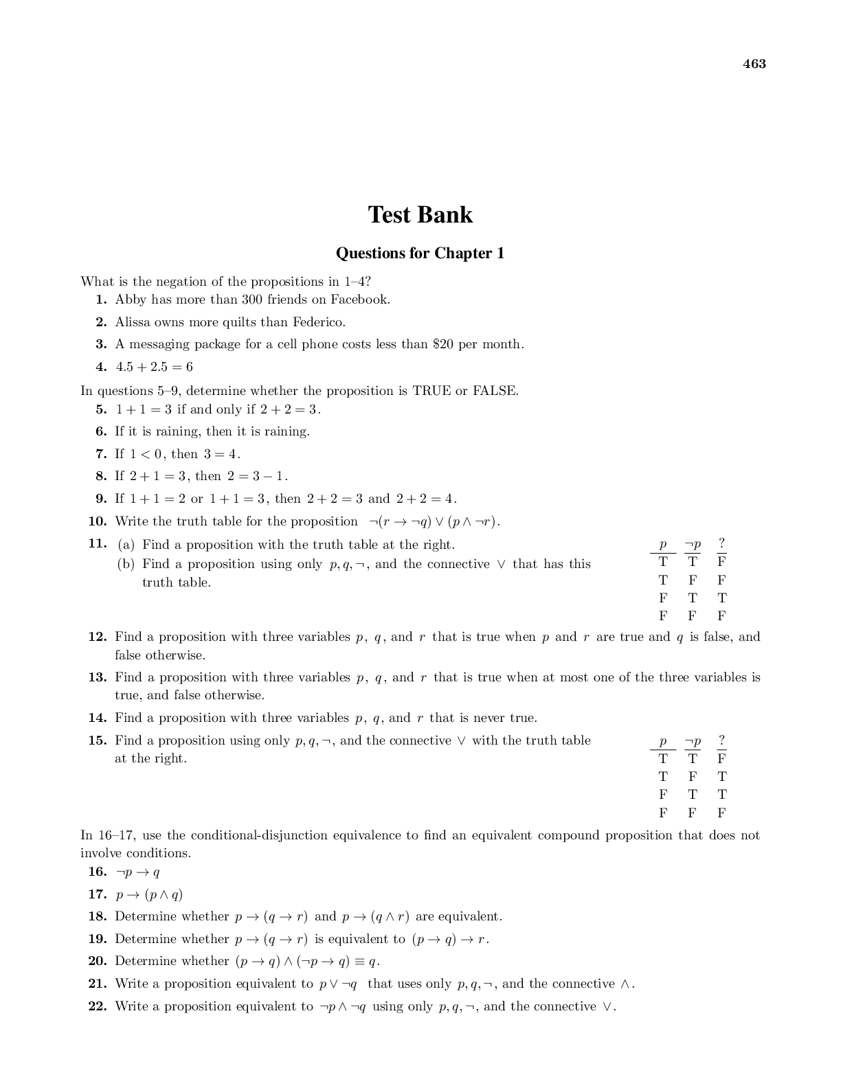
Discrete Mathematics and Its Applications 8th Edition by Kenne...
Finite Mathematics & Its Applications, 13e Larry Goldstein, Da...
Student Solutions Manual for Mathematics for Economics, 4th Ed...