Report for Experiment #13
Simple Harmonic Motion
Lab Partner:
TA:
05/11/16
Abstract
Simple harmonic motions are motions that are described mathematically with the use of cosine functions.
This experiment will atte
...
Report for Experiment #13
Simple Harmonic Motion
Lab Partner:
TA:
05/11/16
Abstract
Simple harmonic motions are motions that are described mathematically with the use of cosine functions.
This experiment will attempt to intimidate simple harmonic motions and dampened harmonic motions
using a frictionless system. The glider is placed on top of an air track attached to two springs on either
side. The glider will either have no magnets (investigation 1) or magnets attached (investigation 2). The
PASCOTM PASPort USB Link and Motion Sensor is used to accurately measure the displacement of the
glider, calculating the amplitude, period, angular frequency, phase and spring constant. When simulating
simple harmonic motion the measured k and the calculated k where within error. This was also the case
the period.
IntroductionThis experiment will test simple harmonic motion and dampened oscillation. This motion can be
summarized by the equation x – x0 = Acos(wt+ ). It is the point of this experiment to investigate ϕ
oscillating motion, by calculating the amplitude A, period T, frequency f, angular frequency w and phase
ϕ. This also includes finding the effects damping forces have on an object in oscillating motion. In the
first investigation we placed a glider on an air track held by springs on either end. First we found the
equilibrium position using the PASCOTM PASPort USB Link and Motion Sensor. We then slide the glider
away from its equilibrium position to create simple harmonic motion. This motion was graphed on
centered position vs time. From this graph we found the height of the first peak which is the amplitude.
We then graph the measured times from the first 6 positive peaks. We then found the slope of this graph
which represents the average period. This is because the period can be viewed as the seconds per peak.
From this we calculated the frequency and the angular frequency. Then using the angular frequency we
calculated the phase . We then calculated the spring constant k ϕ s and compared to the theoretical spring
constant k. The second investigation attached magnets in incremented of 2. At each measurement we
obtain and graph the six peak amplitudes vs the peak times. From this graph we add an exponential trend
line and find the decay constant α. From the decay constant we find the damping constant b. Then then
plot b vs number of magnets for analysis. From this we are able to calculate the period for each of the
runs. We then compare each calculated T to the measured period T.
Investigation 1
Setup & Procedure
The glider is setup on top of the air track. The glider is attached springs on either end. These springs are
attached to the ends of the air track. We use the PASCOTM PASPort USB Link and Motion Sensor to
measure the displacement of the glider. Making sure that the sensor was recording at 20 Hz With the air
on and the glider in almost frictionless state of motion. We allow the glider to come an equilibrium point
and record this position for 30 seconds. We then move the glider toward the motion tracker until the glider
is located at the 50cm mark. We release the glider and records its motion for at least 6 peaks. Ensuring
that this motion had smooth oscillation on its graph. We used this data to analyze simple harmonic
motions.
Table 1 – Equilibium position, wave amplitude, Average period, frequency, angular frequency,
phase, theoretical k, glider mass, calculated k, and peak with time and centered position.
equilibrium position x0 (m) 0.69953
1
wave amplitude A (m) 0.60886
9
Average period T (s) 2.5657
Frequency f (Hz) 0.38975
7
Angular frequency w (rad) 2.44891
7
Phase ϕ -5.02028
Theoretical k' (N/m) 2.2glider mass (Kg) 0.3759
calculated k (N/m) 2.25434
5
peak # Time(s) centered positions (m)
1 2.05 0.608869
2 4.55 0.464669
3 7.15 0.427369
4 9.7 0.397269
5 12.3 0.367969
6 14.85 0.344269
To obtain the equilibrium position x0 we used the average distance that found when we recorded the
glider at equilibrium. Then to find the centered positions we used the equation e.g x – x0 . Then using this
we plotted the centered position vs time as seen in Fig. (1). From this we were able to find the Amplitude
which is the positive peak to the right the y-axis. Using this information we then found the period T using
the measured times from the first 6 positive peaks as seen in Fig. (2). From this graph we used a linear fit
to find the slope. We then used Eq.(13.10) from [1] to find the frequency and angular frequency. We used
the Eq.(13.8) from [1] to find the phase. We are given that the nominal spring constant is ks = 1.1 N/m
knowing that this system is in parallel we find that ks = 2.2 N/m. To find our calculated k = 2.254345 N/m
we used the Eq.(13.7) from [1]. These two k’s are within 3% difference from each other.
[Show More]


.png)

.png)
.png)
.png)

.png)
.png)
.png)


.png)
.png)


.png)


.png)

.png)
