Elements of Statistics. Chapter 1 to chapter 14 Exercise Solutions. All Answers 100% and Explained

Document Content and Description Below

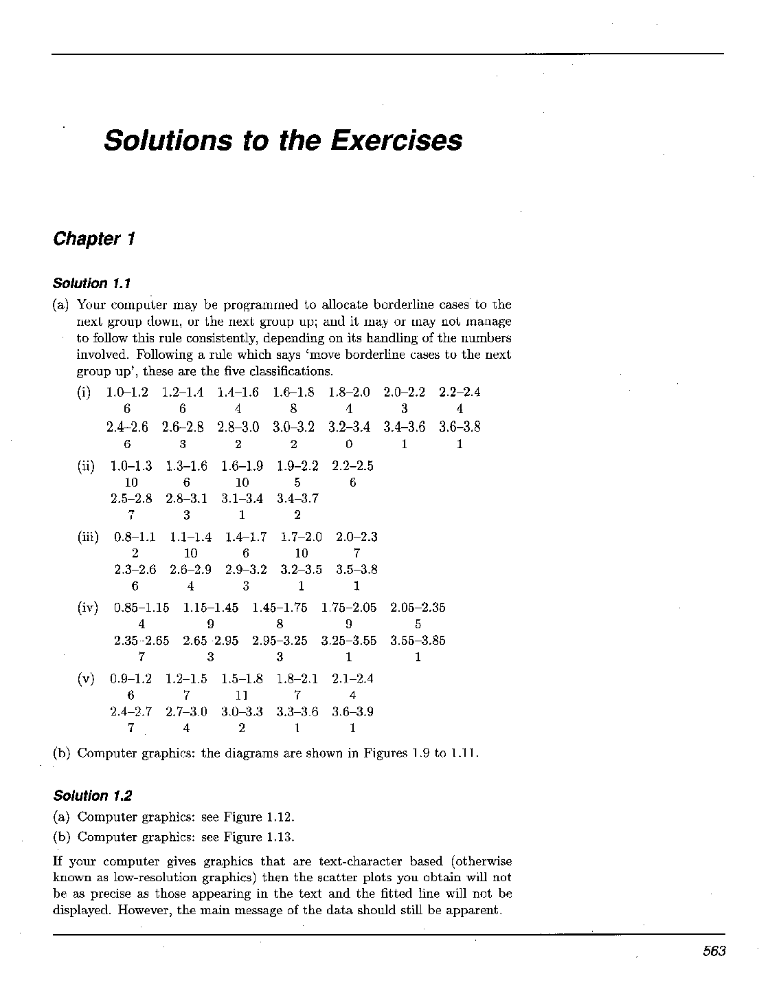
Exercise 1.1 (a) Obtain frequency tables for the SIRDS birth weight data with the following group classifications. (i) 1.0-1.2, 1.2-1.4, . .. (ii) 1.0-1.3, 1.3-1.6, . . . (iii) 0.8-1.1, 1.1-1.4, .... .. (iv) 0.85-1.15, 1.15-1.45, ... (V) 0.9-1.2, 1.2-1.5, . . . (b) Plot histograms for the SIRDS birth weight data with the same group classifications as in part (a). Exercise 1.2 (a) Plot the variable death rate against alcohol consunlption for all fifteen countries, including France, in the data set recording alcohol-related deaths and average individual alcohol consumption. (b) Plot these data points again, excluding France from the data set.Elements of Statistics Exercise 1.3 (a) For the data set recording body and brain weights for different species of animal, sort the species according to decreasing brain weight to body weight ratio. (b) Obtain a scatter plot of brain weight against body weight (i) before and (ii) after a log transformation. Exercise 1.4 Find the median birth weight for the infants who survived, and for those who did not. (Sort the data by hand, rather than using your computer. For data sets much larger than about 30, you will appreciate that hand-sorting becomes impractical.) Exercise 1.5 The first two columns of Table 1.5 give the blood plasma ,B endorphin concentrations of 11 runners before and after the race (successfully completed). There is a marked difference between these concentrations. The data are reproduced in Table 1.11 below with the 'After - Before' difference shown. Table 1 .l 1 Differences in pre- and post-race ,L?endorphin concentration levels Before 4.3 4.6 5.2 5.2 6.6 7.2 8.4 9.0 10.4 14.0 17.8 After 29.6 25.1 15.5 29.6 24.1 37.8 20.2 21.9 14.2 34.6 46.2 Difference 25.3 20.5 10.3 24.4 17.5 30.6 11.8 12.9 3.8 20.6 28.4 Find the median of the 'After - Before' differences given in Table 1.11.Elements o fStatistics Exercise 1.6 The annual snowfall (in inches) in Buffalo, New York, USA was recorded for Parzen, E. (1979) Nonparametric the 63 years from 1910 to 1972. These data are listed in Table 1.12. statistical data modelling. J. American Statistical Association, 74, 105-31. Table 1 . 12 Annual snowfall in Buffalo, NY, 1910-1972 (inches) 126.4 82.4 78.1 51.1 90.9 76.2 104.5 87.4 110.5 25.0 69.3 53.5 39.8 63.6 46.7 72.9 79.7 83.6 80.7 60.3 79.0 74.4 49.6 54.7 71.8 49.1 103.9 51.6 82.4 83.6 77.8 79.3 89.6 85.5 58.0 120.7 110.5 65.4 39.9 40.1 88.7 71.4 83.0 55.9 89.9 84.8 105.2'113.7 124.7 114.5 115.6 102.4 101.4 89.8 71.5 70.9 98.3 55.5 66.1 78.4 120.5 97.0 110.0 Use your computer to find the median annual snowfall over this period. The second representative measure defined in this course for a collection of data is the sample mean. This is simply what most individuals would understand by the word 'average': all the items in the data list are added together, giving the sample total. This number is divided by the number of items (the sample size) The sample mean The mean of a sample is the arithmetic average of the data list, obtained by adding together all of the data values and dividing this total by the number of items in the sample. Denoting the n items in a data set X I , ~ 2 , . .. ,X,, then the sample size is n, and the sample mean is given by - X1+ X2+...+ X,, 1 X = = -EXi. n n i=l The symbol F denoting the sample mean is read 'X-bar'. Example 1.9 continued From the figures in Table 1.5, the mean P endorphin concentration of collapsed runners is where the units of ineasurement are pmol/l. Exercise 1.7 Use your calculator to find the mean birth weight of infants who survived H SIRDS, and of those who died. What was the mean birth weight for the complete sample of 50 infants? Exercise 1.8 Find the mean of the 'After - Before' differences given in Table 1.11.\ Chapter 1 Section 1.3 Exercise 1.9 Use your computer'to find the inean annual snowfall in Buffalo, New York, during the years 1910 to 1972 (see Table 1.12). Two plausible measures have been defined for describing a typical or representative value for a sainple of data. Which measure should be chosen in a statement of that typical value? I11 the examples we have looked at in this section, there has been little to choose between the two. Are there principles that should be followed? It all depends on the data that we are trying to summarize, and our aim in suininarizing them. To a large extent deciding between using the sample inean and the sainple median depends on how the data are distributed. If their distribution appears to be regular and concentrated in the middle of their range, the meail is usually used. It is the easier to coinpute because no sorting is involved, and as you will see later, it is the easier to use for drawing inferences about the population from which the sample has been taken. (Notice the use of the word range here. This is a statement of the extent of the values observed in a sample, as in '. . .the observed weights ranged from a ininiin~unof 1.03kg to a maximum of 3.64 kg'. It need not be an exact statement:' '...the range of observed weights was from l kg to about 4 kg'. However, in Subsection 1.3.2 we shall see the word 'range' used in a technical sense, as a measure of dispersion in data. This often happens in statistics: a familiar word is given a technical meaning. Terms you will coine across later in the course include expect, likelihood, confidence, estimator, significant. But we would not wish this to preclude normal English usage of such words. It will usually be clear from the context when the technical sense is intended.) If, however, the data are irregularly distributed with apparent outliers present, then the sample inedian is usually preferred in quoting a typical value, since it is less sensitive to such irregularities. You can see this by looking again at the data on collapsed runners in Table,1.5. The mean endorphin coilcentration is 138.6 pmol/l, whereas the median concentratioil is 110. The large discrepancy is due to the outlier with an endorphin concentration of 414. Excluding this outlier brings the mean down to 111.1 while the inedian decreases to 106. From this we see that the median is more stable than the inean in the sense that outliers exert less influence upon it. The word resistant is soinetiines used to describe measures which are insensitive to outliers. The median is said to be a resistant measure, whereas the inean is not resistant. The data in Table 1.1 were usefully suininarized in Figure 1.7. The variable recorded here is 'type of employment' (professional, industrial, clerical, and so on) so the data are categorical and not amenable to ordering. In this context the notion of 'mean type of employment' or 'median type of employment' is not a sensible one. For any data set, a third representative measure soinetiines used is the mode, and it describes the most frequently occurring observation. Thus, for males in employment in the USA during 1986, the modal type of employment was 'professional'; while, for females, the modal type of einployinent was 'clerical'. With the help of a computer, neither the sample mean nor the sample median is easier to calculate than the other; but a computer is not always ready to hand. The word m o d e can also reasonably be applied to nuinerical data, referring again to the most frequently occurriilg observation. But there is a problem of definition. For the birth weight data in Table 1.4, there were two duplicates:Elements of Statistics two of the infants weighed 1.72kg, and another two weighed 2.20 kg. So there would appear to be two modes, and yet to report either one of them as a representative weight is to make a great deal of an arithmetic accident. If the data are classified into groups, then we can see from Figures 1.9 to 1.11 that even the definition of a 'modal group' will depend on the definition of borderlines (and on what to do with borderline cases). The number of histogram peaks as well as their locations can alter. However, it often happens that a collection of data presents a very clear picture of an underlying pattern, and one which would be robust against changes in group definition. In such a case it is common to identify as modes not just the most frequently occurring observation (the highest peak) but every peak. Here are two examples. Figure 1.18 shows a histogram of chest measurements (in inches) of a sample of 5732 Scottish soldiers. This data set is explored and discussed in some detail latkr in the course; for the moment, simply observe that there is an evident single mode at around 40 inches. The data are said to be unimodal. Figure 1.19 shows a histogram of waiting times, varying from about 40 nlinutes to about 110 minutes. In fact, these are waiting times between the starts of successive eruptions of the Old Faithful geyser in the Yellowstone National Park, Wyoming, USA, during August, 1985. Observe the two modes. These data are said to be bimodal. Exercise 1.10 (a) Find the lower and upper quartiles for the birth weight data on those children who died of the condition. (See Solution 1.4 for the ordered data.) (b) Find the median, lower and upper quartiles for the data in Table 1.13, which give the percentage of silica found in each of 22 chondrites meteors. (The data are ordered.) Table 1 . 1 3 Silica content of chondrites meteors. 20.77 22.56 22.71 22.99 26.39 27.08 27.32 27.33 27.57 27.81 28.69 29.36 30.25 31.89 32.88 33.23 33.28 33.40 33.52 33.83 33.95 34.82 Good, I.J. and Gaskins, R.A. (1980) Density estimation and bump-hunting by the penalized likelihood method exemplified by scattering and meteorite data. J. American Statistical Association, 75, 42-56. A simple measure of dispersion, the interquartile range, is given by the difference q u - q ~ . I T h e interquartile r a n g e The dispersion in a data set may be simply expressed through the int e r q u a r t i l e range, which is the difference between the upper and lower quartiles, qu - q ~ . Exercise 1.11 Use your conlputer to find the lower and upper quartiles and the interquartile range for the Buffalo snowfall data in Table 1.12. The interquartile range is a useful measure of dispersion in the data and it has the excellent property of not being too sensitive to outlying data values. However, like the median it does suffer from the disadvantage that its computation requires sorting the data. This can be very time-consuming for large samples. Anotller measure that is easier to compute and, as you will find in later chapters, has good statistical properties is the standard deviation. The standard deviation is defined in terms of the differences between the data values and their mean. These differences (xi- c),which can be positive or negative, are called residuals. Example 1.13 Calculating residuals The mean difference in P endorphin coilcentratioil for the 11runners sainpled who completed the Great North Run in Example 1.4 is 18.74 pmol/l (to two decimal places). The eleven residuals are given in the following table. difference,^; 25.3 20.5 10.3 24.4 17.5 30.6 11.8 12.9 3.8 20.6 28.4 Mean, 5 18.74 18.74 18.74 18.74 18.74 18.74 18.74 18.74 18.74 18.74 18.74 Residua1,xi-5 6.56 1.76 -8.44 5.66 -1.24 11.86 .-6.94 -5.84 -14.94 1.86 9.66 ,Elements of Statistics If xi is a data value (i = 1,2,...,n, where n is the sample size) then the ith residual can be written These residuals all contribute to an overall measure of dispersion in the data. Large negative and large positive values both indicate observations far removed from the sample mean. In some way they need to be combined into a single number. There is not much point in averaging them: positive residuals will cancel out negative ones. In fact their sum is zero, since and so, therefore, is their average. What is important is the magnitude of each residual, the absolute difference lxi - 571. The absolute residuals could be added together and averaged, but this measure (known as the mean absolute deviation) does not possess very convenient mathematical properties. Another way of eliminating minus signs is to square the residuals and average them. This leads to a measure of dispersion known as the sample standard deviation. The sample standard deviation A measure of the dispersion in a sample Xlrx21...,Xn with sample mean:is given by the sample standard deviation S , where s is obtained by'averaging the squared residuals, and taking the square root of that average: There are two important points you should note about this definition. First, you should remember to take the square root of the average. The reason for this is that the residuals are measured in the same units as the data, and so their squares are measured in the squares of those units. After averaging, it is necessary to take the square root, so that the standard deviation is measured in the same units as the data. Second, although there are n terms contributing to the sum in the numerator, the divisor is not the sample size n , but n - 1. The reason for this surprising amendment will become clear in Chapter 6 of the course. Either average (dividing conventionally by n or dividing by n - 1) has useful statistical properties, but these properties are subtly different. The definition at (1.1)will be used in this course.Chapter 1 Section 1.3 Example 1.13 continued The sum of the squared residuals for the eleven ,B endorphin concentration differences is so the sample standard deviation of the differences is Notice that a negative residual contributes a positive value to the calculation of the standard deviation. This is because it is squared. Even for relatively small samples the arithmetic is rather awkward if done by hand. Fortunately, it is now common for calculators to have a 'standard deviation' button, and all that is required is to key in the data. Exercise 1.12 Use (a) Confirnl your calculator the sample for each standard of the following deviation calculations. for the 11 differences listed in p Example 1.13. (b) Calculate the standard deviation for the 22 silica percentages given in Table 1.13. (c) Calculate the standard deviation for the ,B endorphin concentrations of the 11 collapsed runners. (See Table 1.5.) Exercise 1.13 Use your computer for each of these calculations. (a) Compute the standard deviation for the birth weights of all 50 infants in a the SIRDS data set. (See Table 1.4.) (b) Find the standard deviation for the annual snowfall in Buffalo, NY. (See Table 1.12.) Exercise 1.14 When hunting insects, bats emit high-frequency sounds and pick up echoes Griffin, D.R., Webster, F.A. and of their prey. The data given in Table 1.14 are bat-to-prey detectioll dis- hlIichael, C.R. (1960) The echo tames (i.e. distances at which the bat first detects the insect) measured in location of 'ying by bats. Animal Behaviour, 8 , 141-154. centimetres. Table 1. l 4 Bat-to-prey detection distances ,(cm) 62 52 68 23 34 45 27 42 83 56 40 Calculate the median, interquartile range, meall and standard deviation of the sample. The Exercise following 1.15data are taken from the 1941 Canadian Census and comprise 8 the sizes of completed families (numbers of children) born to a sample of Protestant mothers in Ontario aged 45-54 and married at age 15-19. The data Keyfitz, N. (1953) A factorial are split into two groups according to how many years of formal education arrangement of com~arisonsof the mothers had received. family size. American J. Sociology, 53, 470-480. Table 1.15 Family size: mothers married aged 15-19 Mother educated for 6 years or less 14 13 4 14 10 2 13 5 0 0 13 3 9 2 10 11 13 5 14 Mother educated for 7 years or more 0 4 0 2 3 3 0 4 7 1 9 4 3 2 3 2 1 6 6 0 1 3 6 6 5 9 1 0 5 4 3 3 5 2 3 5 - 1 5 5 Find the median, interquartile range, mean and standard deviation of each of the groups of mothers. Cominent on these measures for the two groups. For future reference, the square of the sample standard deviation in a sample of data is known as the sample variance. The sample variance The sample variance of a data sample X I , xz, . .. ,X, is given by where is the sample mean. Finally, many practitioners find it convenient and usef~~l to characterize a data sample in terms of the five-figure summary.Chapter 1 Section 1.4 The five-figure summary For a sample of data, the five-figure,summary lists, in order, 0 the sample n~inimum, a the lower quartile, q ~ ; 0 the sample median, m; 0 the upper quartile, qv; 0 the sample maximum, X(,). For instance, the five-figure summary for the snowfall data in Table 1.12 can be written (25,63.6,79.7,98.3,126.4). For the silica data in Table 1.13 it is (20.77,26.91,29.03,33.31,34.82). 1.4 Graphical displays Exercise 1.17 Use your computer to calculate the sample skewness for the family size data for the first group of 19 mothers, who.had six or less years' education. I11 the case of the first group of mothers the sample skewness is negative: the data are said to be negatively skewed. In this case, the asymmetry is rather slight. However, the consequences of asyillinetry are iinportant for subsequent analyses of the data, as we shall see as the course develops. The following exercise is a computer exercise to reinforce some of the ideas you have met so far. Exercise 1.18 Data were taken from an experinlent on three groups of mice. The measurements are amounts of nitrogen-bound bovine serum albumen produced by normal mice treated with a placebo (i.e. an inert substance), alloxan-diabetic mice treated with a placebo, and alloxan-diabetic mice treated with insulin. The data are given in Table 1.16. Table 1.l 6 Nitrogen-based BSA for three groups of diabetic mice Normal Alloxan-diabetic Insulin treatment (a) Sulnmarize the three groups in terms of their five-figure summaries. (b) Calculate the mean and standard deviation for each group. (c) Calculate the sample skewness for each group. (d) Obtain a comparative boxplot for the three groups. Are any differences apparent between the three treatments? [Show More]

Last updated: 2 years ago

Preview 1 out of 105 pages