4.1 Maximum and Minimum Values
1. A function has an absolute minimum at = if () is the smallest function value on the entire domain of , whereas
has a local minimum at if () is the smallest function valu
...
4.1 Maximum and Minimum Values
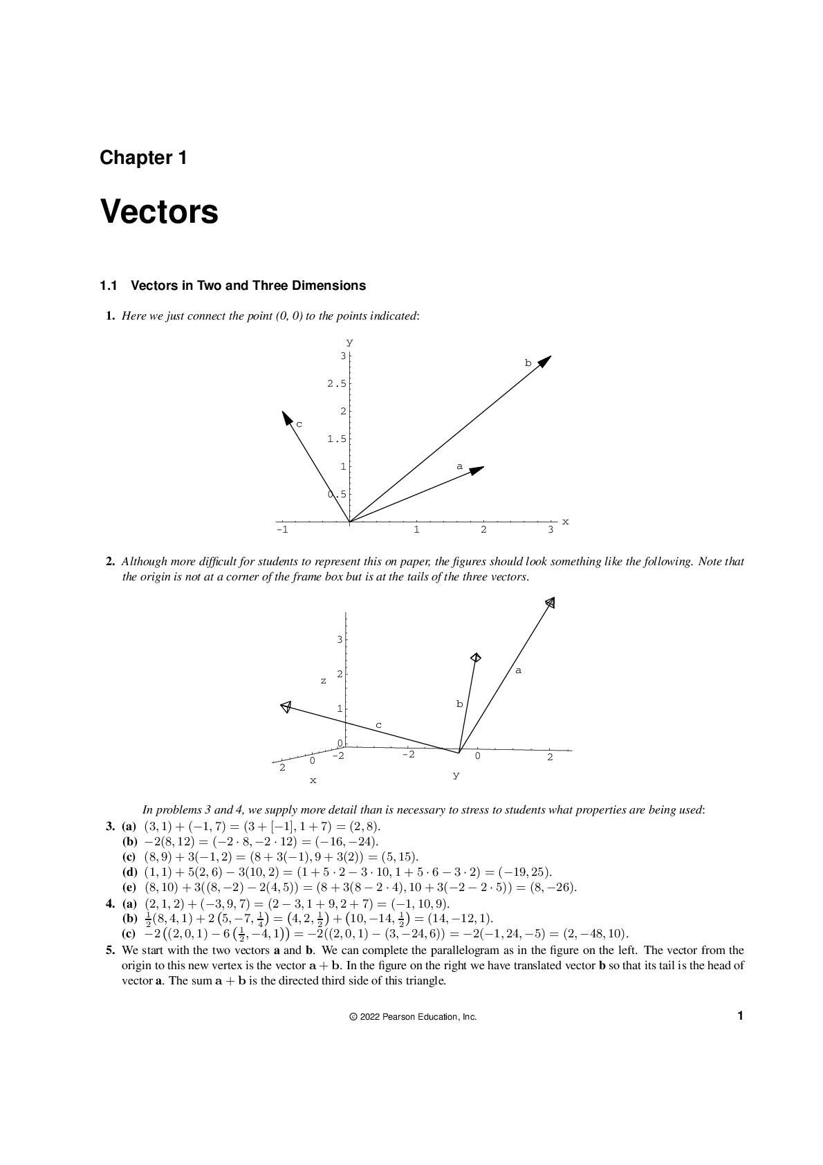
1. A function has an absolute minimum at = if () is the smallest function value on the entire domain of , whereas
has a local minimum at if () is the smallest function value when is near .
2. (a) The Extreme Value Theorem
(b) See the Closed Interval Method.
3. Absolute maximum at , absolute minimum at , local maximum at , local minima at and , neither a maximum nor a
minimum at and .
4. Absolute maximum at ; absolute minimum at ; local maxima at and ; local minimum at ; neither a maximum nor a
minimum at and .
5. Absolute maximum value is (4) = 5; there is no absolute minimum value; local maximum values are (4) = 5 and
(6) = 4; local minimum values are (2) = 2 and (1) = (5) = 3.
6. There is no absolute maximum value; absolute minimum value is (4) = 1; local maximum values are (3) = 4 and
(6) = 3; local minimum values are (2) = 2 and (4) = 1.
7. Absolute maximum at 5, absolute minimum at 2,
local maximum at 3, local minima at 2 and 4
8. Absolute maximum at 4, absolute minimum at 5,
local maximum at 2, local minimum at 3
9. Absolute minimum at 3, absolute maximum at 4,
local maximum at 2
10. Absolute maximum at 2, absolute minimum at 5,
4 is a critial number but there is no local maximum or
minimum there.
°c 2016 Cengage Learning. All Rights Reserved. May not be scanned, copied, or duplicated, or posted to a publicly accessible website, in whole or in part. 1
NOT FOR SALE
INSTRUCTOR USE ONLY
© Cengage Learning. All Rights Reserved.2 ¤ CHAPTER 4 APPLICATIONS OF DIFFERENTIATION
11. (a) (b) (c)
12. (a) Note that a local maximum cannot
occur at an endpoint.
(b)
Note: By the Extreme Value Theorem, must not be continuous.
13. (a) Note: By the Extreme Value Theorem,
must not be continuous; because if it
were, it would attain an absolute
minimum.
(b)
14. (a) (b)
15. () = 1 2(3 − 1), ≤ 3. Absolute maximum
(3) = 4; no local maximum. No absolute or local
minimum.
16. () = 2 − 1 3 , ≥ −2. Absolute maximum
(−2) = 8 3 ; no local maximum. No absolute or local
minimum.
°c 2016 Cengage Learning. All Rights Reserved. May not be scanned, copied, or duplicated, or posted to a publicly accessible website, in whole or in part.
NOT FOR SALE
INSTRUCTOR USE ONLY
© Cengage Learning. All Rights Reserved.SECTION 4.1 MAXIMUM AND MINIMUM VALUES ¤ 3
17. () = 1, ≥ 1. Absolute maximum (1) = 1;
no local maximum. No absolute or local minimum.
18. () = 1, 1 3. No absolute or local maximum.
No absolute or local minimum.
19. () = sin, 0 ≤ 2. No absolute or local
maximum. Absolute minimum (0) = 0; no local
minimum.
20. () = sin, 0 ≤ 2. Absolute maximum
2 = 1; no local maximum. No absolute or local
minimum.
21. () = sin, −2 ≤ ≤ 2. Absolute maximum
2 = 1; no local maximum. Absolute minimum
− 2 = −1; no local minimum.
22. () = cos, − 32 ≤ ≤ 32 . Absolute and local
maximum (0) = 1; absolute and local minima
(± −1).
23. () = ln, 0 ≤ 2. Absolute maximum
(2) = ln 2 ≈ 069; no local maximum. No absolute
or local minimum.
24. () =| |. No absolute or local maximum. Absolute
and local minimum (0) = 0.
°c 2016 Cengage Learning. All Rights Reserved. May not be scanned, copied, or duplicated, or posted to a publicly accessible website, in whole or in part.
NOT FOR SALE
INSTRUCTOR USE ONLY
© Cengage Learning. All Rights Reserved.4 ¤ CHAPTER 4 APPLICATIONS OF DIFFERENTIATION
25. () = 1 − √. Absolute maximum (0) = 1;
no local maximum. No absolute or local minimum.
26. () = . No absolute or local maximum or
minimum value.
27. () = 22− 3 if if −0 1 ≤ ≤≤1 0
No absolute or local maximum.
Absolute minimum (1) = −1; no local minimum.
28. () = 24−+ 1 2 if if 01 ≤≤ ≤ 13
No absolute or local maximum.
Absolute minimum (3) = −2; no local minimum.
29. () = 4 + 1 3 − 1 2 2 ⇒ 0() = 1 3 − . 0() = 0 ⇒ = 1 3 . This is the only critical number.
30. () = 3 + 62 − 15 ⇒ 0() = 32 + 12 − 15 = 3(2 + 4 − 5) = 3( + 5)( − 1).
0() = 0 ⇒ = −5, 1. These are the only critical numbers.
31. () = 23 − 32 − 36 ⇒ 0() = 62 − 6 − 36 = 6(2 − − 6) = 6( + 2)( − 3).
0() = 0 ⇔ = −2, 3. These are the only critical numbers.
32. () = 23 + 2 + 2 ⇒ 0() = 62 + 2 + 2 = 2(32 + + 1). Using the quadratic formula, 0() = 0 ⇔
=
−1 ± √−11
6
. Since the discrimininant, −11, is negative, there are no real soutions, and hence, there are no critical
numbers.
33. () = 4 + 3 + 2 + 1 ⇒ 0() = 43 + 32 + 2 = (42 + 3 + 2). Using the quadratic formula, we see that
42 + 3 + 2 = 0 has no real solution (its discriminant is negative), so 0() = 0 only if = 0. Hence, the only critical number
is 0.
34. () = |3 − 4| = 3 −(3 −4− 4) if if 3 3 − − 4 4 ≥ 0 0 = 34−−34 if if ≥ 4 3 4 3
0() = 3−3 if if 4 3 4 3 and 0() does not exist at = 4 3 , so = 4 3 is a critical number.
°c 2016 Cengage Learning. All Rights Reserved. May not be scanned, copied, or duplicated, or posted to a publicly accessible website, in whole or in part.
NOT FOR SALE
INSTRUCTOR USE ONLY
© Cengage Learning. All Rights Reserved.SECTION 4.1 MAXIMUM AND MINIMUM VALUES ¤ 5
35. () = − 1
2 − + 1 ⇒
0() = (2 − + 1)(1) − ( − 1)(2 − 1)
(2 − + 1)2 =
2 − + 1 − (22 − 3 + 1)
(2 − + 1)2 =
−2 + 2
(2 − + 1)2 =
(2 − )
(2 − + 1)2 .
0() = 0 ⇒ = 0, 2. The expression 2 − + 1 is never equal to 0, so 0() exists for all real numbers.
The critical numbers are 0 and 2.
36. () = − 1
2 + 4 ⇒ 0() = (2 + 4)(1) (2 −+ 4) (2− 1)(2) = 2 + 4 (2−+ 4) 222+ 2 = −(2 2+ 2 + 4) + 4 2 .
0() = 0 ⇒ = −2 ± √4 + 16
−2
= 1 ± √5. The critical numbers are 1 ± √5. [0() exists for all real numbers.]
37. () = 34 − 214 ⇒ 0() = 3 4 −14 − 2 4 −34 = 1 4 −34(312 − 2) = 3√ − 2
4 √4 3 .
0() = 0 ⇒ 3√ = 2 ⇒ √ = 2 3 ⇒ = 4 9 . 0() does not exist at = 0, so the critical numbers are 0 and 4 9 .
38. () = √3 4 − 2 = (4 − 2)13 ⇒ 0() = 1 3(4 − 2)−23(−2) = −2
3(4 − 2)23 . 0() = 0 ⇒ = 0.
0(±2) do not exist. Thus, the three critical numbers are −2, 0, and 2.
39. () = 45( − 4)2 ⇒
0() = 45 · 2( − 4) + ( − 4)2 · 4 5 −15 = 1 5 −15( − 4)[5 · · 2 + ( − 4) · 4]
=
( − 4)(14 − 16)
515 =
2( − 4)(7 − 8)
515
0() = 0 ⇒ = 4, 8 7 . 0(0) does not exist. Thus, the three critical numbers are 0, 8 7 , and 4.
40. () = 4 − tan ⇒ 0() = 4 − sec2 . 0() = 0 ⇒ sec2 = 4 ⇒ sec = ±2 ⇒ cos = ± 1 2 ⇒
=
3 + 2, 53 + 2, 23 + 2, and 43 + 2 are critical numbers.
Note: The values of that make 0() undefined are not in the domain of .
41. () = 2cos + sin2 ⇒ 0() = −2sin + 2sin cos. 0() = 0 ⇒ 2sin (cos − 1) = 0 ⇒ sin = 0
or cos = 1 ⇒ = [ an integer] or = 2. The solutions = include the solutions = 2, so the critical
numbers are = .
42. () = 3 − arcsin ⇒ 0() = 3 − √11− 2 . 0() = 0 ⇒ 3 = √11− 2 ⇒ √1 − 2 = 1 3 ⇒
1 − 2 = 1
9 ⇒ 2 = 8 9 ⇒ = ± 2 3√2 ≈ ±094, both in the domain of , which is [−11].
43. () = 2−3 ⇒ 0() = 2(−3−3) + −3(2) = −3(−3 + 2). 0() = 0 ⇒ = 0, 2 3
[−3 is never equal to 0]. 0() always exists, so the critical numbers are 0 and 2 3 .
44. () = −2 ln ⇒ 0() = −2(1) + (ln)(−2−3) = −3 − 2−3 ln = −3(1 − 2ln) = 1 − 2ln
3 .
0() = 0 ⇒ 1 − 2ln = 0 ⇒ ln = 1 2 ⇒ = 12 ≈ 165. 0(0) does not exist, but 0 is not in the domain
of , so the only critical number is √.
°c 2016 Cengage Learning. All Rights Reserved. May not be scanned, copied, or duplicated, or posted to a publicly accessible website, in whole or in part.
NOT FOR SALE
INSTRUCTOR USE ONLY
© Cengage Learning. All Rights Reserved.6 ¤ CHAPTER 4 APPLICATIONS OF DIFFERENTIATION
45. The graph of 0() = 5−01|| sin − 1 has 10 zeros and exists
everywhere, so has 10 critical numbers.
46. A graph of 0() = 100 cos2
10 + 2 − 1 is shown. There are 7 zeros
between 0 and 10, and 7 more zeros since 0 is an even function.
0 exists everywhere, so has 14 critical numbers.
47. () = 12 + 4 − 2, [05]. 0() = 4 − 2 = 0 ⇔ = 2. (0) = 12, (2) = 16, and (5) = 7.
So (2) = 16 is the absolute maximum value and (5) = 7 is the absolute minimum value.
48. () = 5 + 54 − 23, [04]. 0() = 54 − 62 = 6(9 − 2) = 6(3 + )(3 − ) = 0 ⇔ = −3, 3. (0) = 5,
(3) = 113, and (4) = 93. So (3) = 113 is the absolute maximum value and (0) = 5 is the absolute minimum value.
49. () = 23 − 32 − 12 + 1, [−2 3]. 0() = 62 − 6 − 12 = 6(2 − − 2) = 6( − 2)( + 1) = 0 ⇔
= 2 −1. (−2) = −3, (−1) = 8, (2) = −19, and (3) = −8. So (−1) = 8 is the absolute maximum value and
(2) = −19 is the absolute minimum value.
50. 3 − 62 + 5, [−35]. 0() = 32 − 12 = 3( − 4) = 0 ⇔ = 0, 4. (−3) = −76, (0) = 5, (4) = −27,
and (5) = −20. So (0) = 5 is the absolute maximum value and (−3) = −76 is the absolute minimum value.
51. () = 34 − 43 − 122 + 1, [−23]. 0() = 123 − 122 − 24 = 12(2 − − 2) = 12( + 1)( − 2) = 0 ⇔
= −1, 0, 2. (−2) = 33, (−1) = −4, (0) = 1, (2) = −31, and (3) = 28. So (−2) = 33 is the absolute maximum
value and (2) = −31 is the absolute minimum value.
52. () = (2 − 4)3, [−23]. 0() = 3(2 − 4)2(2) = 6( + 2)2( − 2)2 = 0 ⇔ = −2, 0, 2. (±2) = 0,
(0) = −64, and (3) = 53 = 125. So (3) = 125 is the absolute maximum value and (0) = −64 is the absolute
minimum value.
53. () = + 1
, [024]. 0() = 1 − 1
2 =
2 − 1
2 =
( + 1)( − 1)
2 = 0 ⇔ = ±1, but = −1 is not in the given
interval, [024]. 0() does not exist when = 0, but 0 is not in the given interval, so 1 is the only critical nuumber.
(02) = 52, (1) = 2, and (4) = 425. So (02) = 52 is the absolute maximum value and (1) = 2 is the absolute
minimum value.
54. () =
2 − + 1, [03].
0() = (2 − + 1) − (2 − 1)
(2 − + 1)2 =
2 − + 1 − 22 +
(2 − + 1)2 =
1 − 2
(2 − + 1)2 =
(1 + )(1 − )
(2 − + 1)2 = 0 ⇔
°c 2016 Cengage Learning. All Rights Reserved. May not be scanned, copied, or duplicated, or posted to a publicly accessible website, in whole or in part.
NOT FOR SALE
INSTRUCTOR USE ONLY
© Cengage Learning. All Rights Reserved.SECTION 4.1 MAXIMUM AND MINIMUM VALUES ¤ 7
= ±1, but = −1 is not in the given interval, [03]. (0) = 0, (1) = 1, and (3) = 3 7 . So (1) = 1 is the absolute
maximum value and (0) = 0 is the absolute minimum value.
55. () = − √3 , [−14]. 0() = 1 − 1 3−23 = 1 − 1
323 . 0() = 0 ⇔ 1 = 3123 ⇔ 23 = 13 ⇔
= ±3132 = ±27 1 = ±3√13 = ±√93. 0() does not exist when = 0. (−1) = 0, (0) = 0,
3−√13 = 3−√13 − √−13 = −31 + 3 √3 = 2√93 ≈ 03849, 3√13 = 3√13 − √13 = −2√93, and
(4) = 4 − √3 4 ≈ 2413. So (4) = 4 − √3 4 is the absolute maximum value and √93 = −2√93 is the absolute
minimum value.
56. () =
√
1 + 2 , [02]. 0() = (1 + 2)(1(1 + (2√2)) )2− √(2) = (1 +2√2)−(1 + 2√2√)2(2) = 2√1(1 + − 322)2 .
0() = 0 ⇔ 1 − 32 = 0 ⇔ 2 = 1
3
⇔ = ±√13, but = −√13 is not in the given interval, [02]. 0() does
not exist when = 0, which is an endpoint. (0) = 0, √13 = 1 + 1 1√4 33 = 34−134 = 3344 ≈ 0570, and
(2) =
√2
5
≈ 0283. So √13 = 3344 is the absolute maximum value and (0) = 0 is the absolute minimum value.
57. () = 2 cos + sin 2, [0, 2].
0() = −2sin + cos 2 · 2 = −2sin + 2(1 − 2sin2 ) = −2(2 sin2 + sin − 1) = −2(2 sin − 1)(sin + 1).
0() = 0 ⇒ sin = 1 2 or sin = −1 ⇒ = 6 . (0) = 2, ( 6 ) = √3 + 1 2 √3 = 3 2 √3 ≈ 260, and ( 2 ) = 0.
So ( 6 ) = 3 2 √3 is the absolute maximum value and ( 2 ) = 0 is the absolute minimum value.
58. () = + cot(2), [474]. 0() = 1 − csc2(2) · 1 2 .
0() = 0 ⇒ 1 2 csc2(2) = 1 ⇒ csc2(2) = 2 ⇒ csc(2) = ±√2 ⇒ 1 2 = 4 or 1 2 = 34
4 ≤ ≤ 74 ⇒ 8 ≤ 1 2 ≤ 78 and csc(2) 6= −√2 in the last interval ⇒ = 2 or = 32 .
4 = 4 + cot 8 ≈ 320, 2 = 2 + cot 4 = 2 + 1 ≈ 257, 32 = 32 + cot 32 = 32 − 1 ≈ 371, and
74 = 74 + cot 78 ≈ 308. So 32 = 32 − 1 is the absolute maximum value and 2 = 2 + 1 is the absolute
minimum value.
59. () = −2 ln, 1 24. 0() = −2 · 1
+ (ln)(−2−3) = −3 − 2−3 ln = −3(1 − 2ln) = 1 − 2ln
3 .
0() = 0 ⇔ 1 − 2ln = 0 ⇔ 2ln = 1 ⇔ ln = 1 2 ⇔ = 12 ≈ 165. 0() does not exist
when = 0, which is not in the given interval, 1 24. 1 2 = ln 12
(12)2 =
ln 1 − ln 2
14 = −4ln2 ≈ −2773,
°c 2016 Cengage Learning. All Rights Reserved. May not be scanned, copied, or duplicated, or posted to a publicly accessible website, in whole or in part.
NOT FOR SALE
INSTRUCTOR USE ONLY
© Cengage Learning. All Rights Reserved.8 ¤ CHAPTER 4 APPLICATIONS OF DIFFERENTIATION
12 = (ln112)22 = 12 = 21 ≈ 0184, and (4) = ln4 42 = ln4 16 ≈ 0087. So (12) = 21 is the absolute maximum
value and 1 2 = −4ln2 is the absolute minimum value.
60. () = 2, [−31]. 0() = 2 1 2 + 2(1) = 2 1 2 + 1. 0() = 0 ⇔ 1 2 + 1 = 0 ⇔ = −2.
(−3) = −3−32 ≈ −0669, (−2) = −2−1 ≈ −0736, and (1) = 12 ≈ 1649. So (1) = 12 is the absolute
maximum value and (−2) = −2 is the absolute minimum value.
61. () = ln(2 + + 1), [−11]. 0() = 1
2 + + 1 · (2 + 1) = 0 ⇔ = − 1 2 . Since 2 + + 1 0 for all , the
domain of and 0 is R. (−1) = ln 1 = 0, − 1 2 = ln 3 4 ≈ −029, and (1) = ln 3 ≈ 110. So (1) = ln 3 ≈ 110 is
the absolute maximum value and − 1 2 = ln 3 4 ≈ −029 is the absolute minimum value.
62. () = − 2tan−1 , [04]. 0() = 1 − 2 · 1
1 + 2 = 0 ⇔ 1 = 1 +22 ⇔ 1 + 2 = 2 ⇔ 2 = 1 ⇔
= ±1. (0) = 0, (1) = 1 − 2 ≈ −057, and (4) = 4 − 2tan−1 4 ≈ 135. So (4) = 4 − 2tan−1 4 is the absolute
maximum value and (1) = 1 − 2 is the absolute minimum value.
63. () = (1 − ), 0 ≤ ≤ 1, 0, 0.
0() = · (1 − )−1(−1) + (1 − ) · −1 = −1(1 − )−1[ · (−1) + (1 − ) · ]
= −1(1 − )−1( − − )
At the endpoints, we have (0) = (1) = 0 [the minimum value of ]. In the interval (01), 0() = 0 ⇔ =
+
+ = + 1 − + = ( +) + + − = ( +) · ( +) = ( +)+ .
So + = ( +)+ is the absolute maximum value.
64. The graph of () = 1 + 5 − 3 indicates that 0() = 0 at ≈ ±13 and
that 0() does not exist at ≈ −21, −02, and 23. Those five values of
are the critical numbers of .
65. (a) From the graph, it appears that the absolute maximum value is about
(−077) = 219, and the absolute minimum value is about (077) = 181.
°c 2016 Cengage Learning. All Rights Reserved. May not be scanned, copied, or duplicated, or posted to a publicly accessible website, in whole or in part.
NOT FOR SALE
INSTRUCTOR USE ONLY
© Cengage Learning. All Rights Reserved.SECTION 4.1 MAXIMUM AND MINIMUM VALUES ¤ 9
(b) () = 5 − 3 + 2 ⇒ 0() = 54 − 32 = 2(52 − 3). So 0() = 0 ⇒ = 0, ± 3 5 .
− 3 5 = − 3 5 5 − − 3 5 3 + 2 = − 3 52 3 5 + 3 5 3 5 + 2
= 3 5 − 25 9 3 5 + 2 = 25 6 3 5 + 2 (maximum)
and similarly, 3 5 = − 25 6 3 5 + 2 (minimum).
66. (a) From the graph, it appears that the absolute maximum value
is about (1) = 285, and the absolute minimum value is about
(023) = 189.
(b) () = + −2 ⇒ 0() = − 2−2 = −2(3 − 2). So 0() = 0 ⇔ 3 = 2 ⇔ 3 = ln 2 ⇔
= 1
3 ln 2 [≈ 023]. 1 3 ln 2 = (ln 2)13 + (ln 2)−23 = 213 + 2−23 [≈ 189], the minimum value.
(1) = 1 + −2 [≈ 285], the maximum.
67. (a) From the graph, it appears that the absolute maximum value is about
(075) = 032, and the absolute minimum value is (0) = (1) = 0;
that is, at both endpoints.
(b) () = √ − 2 ⇒ 0() = · 1 − 2
2√ − 2 + √ − 2 = ( − 222√) + (2 − 2− 22) = 23√ −−422 .
So 0() = 0 ⇒ 3 − 42 = 0 ⇒ (3 − 4) = 0 ⇒ = 0 or 3 4 .
(0) = (1) = 0 (minimum), and 3 4 = 3 4 3 4 − 3 42 = 3 4 16 3 = 316 √3 (maximum).
68. (a) From the graph, it appears that the absolute maximum value is about
(−2) = −117, and the absolute minimum value is about
(−052) = −226.
(b) () = − 2cos ⇒ 0() = 1 + 2 sin. So 0() = 0 ⇒ sin = − 1 2 ⇒ = − 6 on [−20].
(−2) = −2 − 2cos(−2) (maximum) and − 6 = − 6 − 2cos− 6 = − 6 − 2 √23 = − 6 − √3 (minimum).
69. Let = 135 and = −2802. Then () = ⇒ 0() = ( · + · 1) = ( + 1). 0() = 0 ⇔
+ 1 = 0 ⇔ = −1
≈ 036 h. (0) = 0, (−1) = − −1 = − ≈ 0177, and (3) = 33 ≈ 00009. The
maximum average BAC during the first three hours is about 0177 mgmL and it occurs at approximately 036 h (214 min).
°c 2016 Cengage Learning. All Rights Reserved. May not be scanned, copied, or duplicated, or posted to a publicly accessible website, in whole or in part.
NOT FOR SALE
INSTRUCTOR USE ONLY
© Cengage Learning. All Rights Reserved.10 ¤ CHAPTER 4 APPLICATIONS OF DIFFERENTIATION
70. () = 8(−04 − −06) ⇒ 0() = 8(−04−04 + 06−06). 0() = 0 ⇔ 06−06 = 04−04 ⇔
06
04 = −04+06 ⇔ 3 2 = 02 ⇔ 02 = ln 3 2 ⇔ = 5ln 3 2 ≈ 2027 h. (0) = 8(1 − 1) = 0,
5ln 3 2 = 8(−2 ln 32 − −3 ln 32) = 8 3 2 −2 − 3 2 −3 = 8 4 9 − 27 8 = 32 27 ≈ 1185, and
(12) = 8(−48 − −72) ≈ 0060. The maximum concentration of the antibiotic during the first 12 hours is 32 27 gmL.
71. The density is defined as = mass
volume =
1000
() (in gcm3). But a critical point of will also be a critical point of
[since
= −1000 −2 and is never 0], and is easier to differentiate than .
() = 99987 − 006426 + 00085043 2 − 00000679 3 ⇒ 0() = −006426 + 00170086 − 00002037 2.
Setting this equal to 0 and using the quadratic formula to find , we get
= −00170086 ± √001700862 − 4 · 00002037 · 006426
2(−00002037) ≈ 39665◦C or 795318◦C. Since we are only interested
in the region 0◦C ≤ ≤ 30◦C, we check the density at the endpoints and at 39665◦C: (0) ≈ 1000
99987 ≈ 100013;
(30) ≈ 1000
10037628 ≈ 099625; (39665) ≈ 999 1000 7447 ≈ 1000255. So water has its maximum density at
about 39665◦C.
72. =
sin + cos ⇒
=
(sin + cos)(0) − (cos − sin)
(sin + cos)2 =
−(cos − sin)
(sin + cos)2 .
So
= 0 ⇒ cos − sin = 0 ⇒ = cos sin = tan. Substituting tan for in gives us
= (tan)
(tan)sin + cos =
tan
sin2
cos + cos
=
tan cos
sin2 + cos2 =
sin
1
= sin.
If tan = , then sin = 2 + 1 (see the figure), so = 2 + 1.
We compare this with the value of at the endpoints: (0) = and 2 = .
Now because 2 + 1 ≤ 1 and 2 + 1 ≤ , we have that 2 + 1is less than or equal to each of (0) and 2 .
Hence, 2 + 1 is the absolute minimum value of (), and it occurs when tan = .
73. () = 0014413 − 041772 + 2703 + 10601 ⇒ 0() = 0043232 − 08354 + 2703. Use the quadratic formula
to solve 0() = 0. = 08354 ± (08354)2 − 4(004323)(2703)
2(004323) ≈ 41 or 152. For 0 ≤ ≤ 12, we have
(0) = 10601, (41) ≈ 10652, and (12) ≈ 10573. Thus, the water level was highest during 2012 about 41 months
after January 1.
°c 2016 Cengage Learning. All Rights Reserved. May not be scanned, copied, or duplicated, or posted to a publicly accessible website, in whole or in part.
NOT FOR SALE
INSTRUCTOR USE ONLY
© Cengage Learning. All Rights Reserved.SECTION 4.1 MAXIMUM AND MINIMUM VALUES ¤ 11
74. (a) The equation of the graph in the figure is
() = 0001463 − 0115532 + 2498169 − 2126872.
(b) () = 0() = 0004382 − 023106 + 2498169 ⇒
0() = 000876 − 023106.
0() = 0 ⇒ 1 = 0 0 23106 00876 ≈ 264. (0) ≈ 2498, (1) ≈ 2193,
and (125) ≈ 6454.
The maximum acceleration is about 645 fts2 and the minimum acceleration is about 2193 fts2.
75. (a) () = (0 − )2 = 02 − 3 ⇒ 0() = 20 − 32. 0() = 0 ⇒ (20 − 3) = 0 ⇒
= 0 or 2
3 0 (but 0 is not in the interval). Evaluating at 1 2 0, 2 3 0, and 0, we get 1 2 0 = 1 8 03, 2 3 0 = 27 4 03,
and (0) = 0. Since 27 4 1 8 , attains its maximum value at = 2 3 0. This supports the statement in the text.
(b) From part (a), the maximum value of is 27 4 03. (c)
76. () = 2 + ( − 5)3 ⇒ 0() = 3( − 5)2 ⇒ 0(5) = 0, so 5 is a critical number. But (5) = 2 and takes on
values 2 and values 2 in any open interval containing 5, so does not have a local maximum or minimum at 5.
77. () = 101 + 51 + + 1 ⇒ 0() = 101100 + 5150 + 1 ≥ 1 for all , so 0() = 0 has no solution. Thus, ()
has no critical number, so () can have no local maximum or minimum.
78. Suppose that has a minimum value at , so () ≥ () for all near . Then () = −() ≤ −() = () for all
near , so () has a maximum value at .
79. If has a local minimum at , then () = −() has a local maximum at , so 0() = 0 by the case of Fermat’s Theorem
proved in the text. Thus, 0() = −0() = 0.
80. (a) () = 3 + 2 + + , 6= 0. So 0() = 32 + 2 + is a quadratic and hence has either 2, 1, or 0 real roots,
so () has either 2, 1 or 0 critical numbers.
Case (i) [2 critical numbers]: () = 3 − 3 ⇒
0() = 32 − 3, so = −1, 1
are critical numbers.
°c 2016 Cengage Learning. All Rights Reserved. May not be scanned, copied, or duplicated, or posted to a publicly accessible website, in whole or in part.
NOT FOR SALE
INSTRUCTOR USE ONLY
© Cengage Learning. All Rights Reserved.12 ¤ CHAPTER 4 APPLICATIONS OF DIFFERENTIATION
Case (ii) [1 critical number]: () = 3 ⇒
0() = 32, so = 0
is the only critical number.
Case (iii) [no critical number]: () = 3 + 3 ⇒
0() = 32 + 3,
so there is no critical number.
(b) Since there are at most two critical numbers, it can have at most two local extreme values and by (i) this can occur. By (iii)
it can have no local extreme value. However, if there is only one critical number, then there is no local extreme value.
APPLIED PROJECT The Calculus of Rainbows
1. From Snell’s Law, we have sin = sin ≈ 4 3 sin ⇔ ≈ arcsin 3 4 sin. We substitute this into
() = + 2 − 4 = + 2 − 4arcsin 3 4 sin, and then differentiate to find the minimum:
0() = 2 − 41 − 3 4 sin2−12 3 4 cos = 2 − 1 −3cos 16 9 sin 2 . This is 0 when 1 −3cos 16 9 sin 2 = 2 ⇔
9 4
cos2 = 1 − 9
16 sin2 ⇔ 9 4 cos2 = 1 − 16 9 1 − cos2 ⇔ 27 16 cos2 = 16 7 ⇔ cos = 27 7 ⇔
= arccos 27 7 ≈ 594◦, and so the local minimum is (594◦) ≈ 24 radians ≈ 138◦.
To see that this is an absolute minimum, we check the endpoints, which in this case are = 0 and = 2 :
(0) = radians = 180◦, and 2 ≈ 166◦.
Another method: We first calculate
: sin = 4 3 sin ⇔ cos = 4 3 cos ⇔ = 34 cos cos , so since
0() = 2 − 4
= 0 ⇔ = 12, the minimum occurs when 3cos = 2cos. Now we square both sides and
substitute sin = 4
3 sin, leading to the same result.
2. If we repeat Problem 1 with in place of 4 3 , we get () = + 2 − 4arcsin1 sin ⇒
0() = 2 − 4cos
1 − sin 2 , which is 0 when 2cos = 1 − sin 2 ⇔ 2cos 2 = 1 − sin 2 ⇔
4cos2 = 2 − sin2 ⇔ 3cos2 = 2 − 1 ⇔ = arccos 23− 1. So for ≈ 13318 (red light) the minimum
°c 2016 Cengage Learning. All Rights Reserved. May not be scanned, copied, or duplicated, or posted to a publicly accessible website, in whole or in part.
NOT FOR SALE
INSTRUCTOR USE ONLY
© Cengage Learning. All Rights Reserved.APPLIED PROJECT THE CALCULUS OF RAINBOWS ¤ 13
occurs at 1 ≈ 1038 radians, and so the rainbow angle is about − (1) ≈ 423◦. For ≈ 13435 (violet light) the
minimum occurs at 2 ≈ 1026 radians, and so the rainbow angle is about − (2) ≈ 406◦.
Another method: As in Problem 1, we can instead find 0() in terms of
, and then substitute = cos cos .
3. At each reflection or refraction, the light is bent in a counterclockwise direction: the bend at is − , the bend at is
− 2, the bend at is again − 2, and the bend at is − . So the total bend is
() = 2( − ) + 2( − 2) = 2 − 6 + 2, as required. We substitute = arcsinsin and differentiate, to get
0() = 2 − 6cos
1 − sin2 , which is 0 when 3cos = 1 − sin2 ⇔ 9cos2 = 2 − sin2 ⇔
8cos2 = 2 − 1 ⇔ cos = 1 8(2 − 1). If = 4 3 , then the minimum occurs at
1 = arccos(43)82 − 1 ≈ 1254 radians. Thus, the minimum
counterclockwise rotation is (1) ≈ 231◦, which is equivalent to a
clockwise rotation of 360◦ − 231◦ = 129◦ (see the figure). So the rainbow
angle for the secondary rainbow is about 180◦ − 129◦ = 51◦, as required.
In general, the rainbow angle for the secondary rainbow is
− [2 − ()] = () − .
4. In the primary rainbow, the rainbow angle gets smaller as gets larger, as we found in Problem 2, so the colors appear from
top to bottom in order of increasing . But in the secondary rainbow, the rainbow angle gets larger as gets larger. To see this,
we find the minimum deviations for red light and for violet light in the secondary rainbow. For ≈ 13318 (red light) the
minimum occurs at 1 ≈ arccos13318 82 − 1 ≈ 1255 radians, and so the rainbow angle is (1) − ≈ 506◦. For
≈ 13435 (violet light) the minimum occurs at 2 ≈ arccos13435 82 − 1 ≈ 1248 radians, and so the rainbow angle is
(2) − ≈ 536◦. Consequently, the rainbow angle is larger for colors with higher indices of refraction, and the colors
appear from bottom to top in order of increasing , the reverse of their order in the primary rainbow.
Note that our calculations above also explain why the secondary rainbow is more spread out than the primary rainbow: in
the primary rainbow, the difference between rainbow angles for red and violet light is about 17◦, whereas in the secondary
rainbow it is about 3◦.
°c 2016 Cengage Learning. All Rights Reserved. May not be scanned, copied, or duplicated, or posted to a publicly accessible website, in whole or in part.
NOT FOR SALE
INSTRUCTOR USE ONLY
© Cengage Learning. All Rights Reserved.14 ¤ CHAPTER 4 APPLICATIONS OF DIFFERENTIATION
4.2 The Mean Value Theorem
1. (1) is continuous on the closed interval [08].
(2) is differentiable on the open interval (08).
(3) (0) = 3 and (8) = 3
Thus, statisfies the hypotheses of Rolle’s Theorem. The numbers = 1 and = 5 satisfy the conclusion of Rolle’s Theorem
since 0(1) = 0(5) = 0.
2. The possible graphs fall into two general categories: (1) Not continuous and therefore not differentiable, (2) Continuous, but
not differentiable.
In either case, there is no number such that 0() = 0.
3. (a) (1) is continuous on the closed interval [08].
(2) is differentiable on the open interval (08).
(b) 0() = (8) − (0)
8 − 0
=
4 − 1
8
=
3 8
.
It appears that 0() = 3 8 when ≈ 22 and 64.
(c) 0() = (6) − (2)
6 − 2
=
1 − 3
4 = −
1 2
.
It appears that 0() = − 1 2 when ≈ 37 and 55.
4. The function shown in the figure is continuous on [08] [but not
differentiable on (08)] with (0) = 1 and (8) = 4. The line
passing through the two points has slope 3 8. There is no number in
(0 8) such that 0() = 3 8.
5. () = 22 − 4 + 5, [−1 3]. is a polynomial, so it’s continuous and differentiable on R, and hence, continuous
on [−13] and differentiable on (−1 3). Since (−1) = 11 and (3) = 11, satisfies all the hypotheses of Rolle’s
°c 2016 Cengage Learning. All Rights Reserved. May not be scanned, copied, or duplicated, or posted to a publicly accessible website, in whole or in part.
NOT FOR SALE
INSTRUCTOR USE ONLY
© Cengage Learning. All Rights Reserved.SECTION 4.2 THE MEAN VALUE THEOREM ¤ 15
Theorem. 0() = 4 − 4 and 0() = 0 ⇔ 4 − 4 = 0 ⇔ = 1. = 1 is in the interval (−13), so 1 satisfies the
conclusion of Rolle’s Theorem.
6. () = 3 − 22 − 4 + 2, [−22]. is a polynomial, so it’s continuous and differentiable on R, and hence, continuous on
[−22] and differentiable on (−2 2). Since (−2) = −6 and (2) = −6, satisfies all the hypotheses of Rolle’s Theorem.
0() = 32 − 4 − 4 and 0() = 0 ⇔ (3 + 2)( − 2) = 0 ⇔ = − 2 3 or 2. = − 2 3 is in the open interval
(−22) (but 2 isn’t), so only − 2 3 satisfies the conclusion of Rolle’s Theorem.
7. () = sin(2), [232]. , being the composite of the sine function and the polynomial 2, is continuous and
differentiable on R, so it is continuous on [2 32] and differentiable on (232). Also, 2 = 1 2√2 = 32 .
0() = 0 ⇔ 1 2 cos(2) = 0 ⇔ cos(2) = 0 ⇔ 2 = 2 + ⇔ = + 2, an integer.
Only = is in (2 32), so satisfies the conclusion of Rolle’s Theorem.
8. () = + 1, 1 2 2. 0() = 1 − 12 = 2 − 1
2 . is a rational function that is continuous on its domain,
(−∞0) ∪ (0 ∞), so it is continuous on 1 2 2. 0 has the same domain and is differentiable on 1 2 2. Also,
1 2 = 5 2 = (2). 0() = 0 ⇔ 2 − 1
2 = 0 ⇔ 2 − 1 = 0 ⇔ = ±1. Only 1 is in 1 2 2 so 1 satisfies the
conclusion of Rolle’s Theorem.
9. () = 1 − 23. (−1) = 1 − (−1)23 = 1 − 1 = 0 = (1). 0() = − 2 3 −13, so 0() = 0 has no solution. This
does not contradict Rolle’s Theorem, since 0(0) does not exist, and so is not differentiable on (−11).
10. () = tan. (0) = tan 0 = 0 = tan = (). 0() = sec2 ≥ 1, so 0() = 0 has no solution. This does not
contradict Rolle’s Theorem, since 0 2 does not exist, and so is not differentiable on (0 ). (Also, () is not continuous
on [0 ].)
11. () = 22 − 3 + 1, [02]. is continuous on [02] and differentiable on (02) since polynomials are continuous and
differentiable on R. 0() = () − ()
− ⇔ 4 − 3 = (2) 2 −− 0(0) = 3 −2 1 = 1 ⇔ 4 = 4 ⇔ = 1, which
is in (0 2)
12. () = 3 − 3 + 2, [−22]. is continuous on [−22] and differentiable on (−22) since polynomials are continuous and
differentiable on R. 0() = () − ()
− ⇔ 32 − 3 = (2) 2 −−( −(2) −2) = 4 −4 0 = 1 ⇔ 32 = 4 ⇔
2 = 4
3
⇔ = ±√23, which are both in (−22).
13. () = ln, [14]. is continuous and differentiable on (0 ∞), so is continuous on [14] and differentiable on (14).
0() = () − ()
− ⇔
1
=
(4) − (1)
4 − 1 =
ln 4 − 0
3
=
ln 4
3
⇔ =
3
ln 4 ≈ 216, which is in (14).
°c 2016 Cengage Learning. All Rights Reserved. May not be scanned, copied, or duplicated, or posted to a publicly accessible website, in whole or in part.
NOT FOR SALE
INSTRUCTOR USE ONLY
© Cengage Learning. All Rights Reserved.16 ¤ CHAPTER 4 APPLICATIONS OF DIFFERENTIATION
14. () = 1
, [13]. is continuous and differentiable on (−∞0) ∪ (0 ∞), so is continous on [1 3] and differentiable
on (13). 0() = () − ()
− ⇔ −
1 2
=
(3) − (1)
3 − 1
=
1 3
− 1
2
= −
1 3
⇔ 2 = 3 ⇔ = ±√3, but only √3
is in (1 3).
15. () = √, [0 4]. 0() = (4) − (0)
4 − 0 ⇔
1
2√ =
2 − 0
4 ⇔
1
2√ =
1 2
⇔ √ = 1 ⇔ = 1. The secant line and the tangent line
are parallel.
16. () = −, [02]. 0() = (2) − (0)
2 − 0
⇔ −− = −2 − 1
2
⇔
− = 1 − −2
2
⇔ − = ln 1 − −2
2
⇔
= −ln 1 − −2
2
≈ 08386. The secant line and the tangent line are
parallel.
17. () = ( − 3)−2 ⇒ 0() = −2( − 3)−3. (4) − (1) = 0()(4 − 1) ⇒ 1
12 −
1
(−2)2 =
−2
( − 3)3 · 3 ⇒
3 4
=
−6
( − 3)3 ⇒ ( − 3)3 = −8 ⇒ − 3 = −2 ⇒ = 1, which is not in the open interval (1 4). This does not
contradict the Mean Value Theorem since is not continuous at = 3.
18. () = 2 − |2 − 1| = 2 2 − − (2 [−(2−1) − 1)] if if 2 2 − − 1 1 ≥ 0 0 = 31 + 2 − 2 if if ≥ 1 2 1 2 ⇒ 0() = −22 if if 1 21 2
(3) − (0) = 0()(3 − 0) ⇒ −3 − 1 = 0() · 3 ⇒ 0() = − 4 3 [not ± 2]. This does not contradict the Mean
Value Theorem since is not differentiable at = 1 2 .
19. Let () = 2 + cos. Then (−) = −2 − 1 0 and (0) = 1 0. Since is the sum of the polynomial 2 and the
trignometric function cos, is continuous and differentiable for all . By the Intermediate Value Theorem, there is a number
in (−0) such that () = 0. Thus, the given equation has at least one real root. If the equation has distinct real roots and
with , then () = () = 0. Since is continuous on [ ] and differentiable on ( ), Rolle’s Theorem implies that
there is a number in ( ) such that 0() = 0. But 0() = 2 − sin 0 since sin ≤ 1. This contradiction shows that the
given equation can’t have two distinct real roots, so it has exactly one root.
20. Let () = 3 + . Then (−1) = −1 + 1 0 and (0) = 1 0. Since is the sum of a polynomial and the natural
exponential function, is continous and differentiable for all . By the Intermediate Value Theorem, there is a number in
(−10) such that () = 0. Thus, the given equation has at least one real root. If the equation has distinct real roots and
°c 2016 Cengage Learning. All Rights Reserved. May not be scanned, copied, or duplicated, or posted to a publicly accessible website, in whole or in part.
NOT FOR SALE
INSTRUCTOR USE ONLY
© Cengage Learning. All Rights Reserved.SECTION 4.2 THE MEAN VALUE THEOREM ¤ 17
with , then () = () = 0. Since is continuous on [ ] and differentiable on ( ), Rolle’s Theorem implies that
there is a number in ( ) such that 0() = 0. But 0() = 32 + 0. This contradiction shows that the given equation
can’t have two distinct real roots, so it has exactly one root.
21. Let () = 3 − 15 + for in [−2 2]. If has two real roots and in [−2 2], with , then () = () = 0. Since
the polynomial is continuous on [ ] and differentiable on ( ), Rolle’s Theorem implies that there is a number in ( )
such that 0() = 0. Now 0() = 32 − 15. Since is in ( ), which is contained in [−22], we have || 2, so 2 4.
It follows that 32 − 15 3 · 4 − 15 = −3 0. This contradicts 0() = 0, so the given equation can’t have two real roots
in [−22]. Hence, it has at most one real root in [−22].
22. () = 4 + 4 + . Suppose that () = 0 has three distinct real roots , , where . Then
() = () = () = 0. By Rolle’s Theorem there are numbers 1 and 2 with 1 and 2
and 0 = 0(1) = 0(2), so 0() = 0 must have at least two real solutions. However
0 = 0() = 43 + 4 = 4(3 + 1) = 4( + 1)(2 − + 1) has as its only real solution = −1. Thus, () can have at
most two real roots.
23. (a) Suppose that a cubic polynomial () has roots 1 2 3 4, so (1) = (2) = (3) = (4).
By Rolle’s Theorem there are numbers 1, 2, 3 with 1 1 2, 2 2 3 and 3 3 4 and
0(1) = 0(2) = 0(3) = 0. Thus, the second-degree polynomial 0() has three distinct real roots, which is
impossible.
(b) We prove by induction that a polynomial of degree has at most real roots. This is certainly true for = 1. Suppose
that the result is true for all polynomials of degree and let () be a polynomial of degree + 1. Suppose that () has
more than + 1 real roots, say 1 2 3 · · · +1 +2. Then (1) = (2) = · · · = (+2) = 0.
By Rolle’s Theorem there are real numbers 1 +1 with 1 1 2 +1 +1 +2 and
0(1) = · · · = 0(+1) = 0. Thus, the th degree polynomial 0() has at least + 1 roots. This contradiction shows
that () has at most + 1 real roots.
24. (a) Suppose that () = () = 0 where . By Rolle’s Theorem applied to on [ ] there is a number such that
and 0() = 0.
(b) Suppose that () = () = () = 0 where . By Rolle’s Theorem applied to () on [ ] and [ ] there are
numbers and with 0() = 0 and 0() = 0. By Rolle’s Theorem applied to 0() on [ ] there is a
number with such that 00() = 0.
(c) Suppose that is times differentiable on R and has + 1 distinct real roots. Then () has at least one real root.
25. By the Mean Value Theorem, (4) − (1) = 0()(4 − 1) for some ∈ (1 4). But for every ∈ (14) we have
0() ≥ 2. Putting 0() ≥ 2 into the above equation and substituting (1) = 10, we get
(4) = (1) + 0()(4 − 1) = 10 + 3 0() ≥ 10 + 3 · 2 = 16. So the smallest possible value of (4) is 16.
°c 2016 Cengage Learning. All Rights Reserved. May not be scanned, copied, or duplicated, or posted to a publicly accessible website, in whole or in part.
NOT FOR SALE
INSTRUCTOR USE ONLY
© Cengage Learning. All Rights Reserved.18 ¤ CHAPTER 4 APPLICATIONS OF DIFFERENTIATION
26. If 3 ≤ 0() ≤ 5 for all , then by the Mean Value Theorem, (8) − (2) = 0() · (8 − 2) for some in [28].
( is differentiable for all , so, in particular, is differentiable on (28) and continuous on [2 8]. Thus, the hypotheses
of the Mean Value Theorem are satisfied.) Since (8) − (2) = 6 0() and 3 ≤ 0() ≤ 5, it follows that
6 · 3 ≤ 6 0() ≤ 6 · 5 ⇒ 18 ≤ (8) − (2) ≤ 30
27. Suppose that such a function exists. By the Mean Value Theorem there is a number 0 2 with
0() = (2) − (0)
2 − 0
=
5 2
. But this is impossible since 0() ≤ 2 5 2 for all , so no such function can exist.
28. Let = − . Note that since () = (), () = () − () = 0. Then since and are continuous on [ ] and
differentiable on ( ), so is , and thus satisfies the assumptions of the Mean Value Theorem. Therefore, there is
a number with such that () = () − () = 0()( − ). Since 0() 0, 0()( − ) 0, so
() − () = () 0 and hence () ().
29. Consider the function () = sin, which is continuous and differentiable on R. Let be a number such that 0 2.
Then is continuous on [0 ] and differentiable on (0 ). By the Mean Value Theorem, there is a number in (0 ) such that
() − (0) = 0()( − 0); that is, sin − 0 = (cos )(). Now cos 1 for 0 2, so sin 1 · = . We took
to be an arbitrary number in (0 2), so sin for all satisfying 0 2.
30. satisfies the conditions for the Mean Value Theorem, so we use this theorem on the interval [− ]: () − (−)
− (−) = 0()
for some ∈ (− ). But since is odd, (−) = −(). Substituting this into the above equation, we get
() + ()
2 = 0() ⇒ () = 0().
31. Let () = sin and let . Then () is continuous on [ ] and differentiable on ( ). By the Mean Value Theorem,
there is a number ∈ ( ) with sin − sin = () − () = 0()( − ) = (cos)( − ). Thus,
|sin − sin| ≤ |cos| | − | ≤ | − |. If , then |sin − sin| = |sin − sin| ≤ | − | = | − |. If = , both
sides of the inequality are 0.
32. Suppose that 0() = . Let () = , so 0() = . Then, by Corollary 7, () = () + , where is a constant, so
() = + .
33. For 0, () = (), so 0() = 0(). For 0, 0() = (1)0 = −12 and 0() = (1 + 1)0 = −12, so
again 0() = 0(). However, the domain of () is not an interval [it is (−∞ 0) ∪ (0 ∞)] so we cannot conclude that
− is constant (in fact it is not).
34. Let () = 2 sin−1 − cos−1(1 − 22). Then 0() = √1 2− 2 − 1 − (1 4− 22)2 = √1 2− 2 − 2 √41− 2 = 0
[since ≥ 0]. Thus, 0() = 0 for all ∈ (01). Thus, () = on (01). To find , let = 05. Thus,
2sin−1(05) − cos−1(05) = 2 6 − 3 = 0 = . We conclude that () = 0 for in (01). By continuity of , () = 0
on [0 1]. Therefore, we see that () = 2 sin−1 − cos−1(1 − 22) = 0 ⇒ 2 sin−1 = cos−1(1 − 22).
°c 2016 Cengage Learning. All Rights Reserved. May not be scanned, copied, or duplicated, or posted to a publicly accessible website, in whole or in part.
NOT FOR SALE
INSTRUCTOR USE ONLY
© Cengage Learning. All Rights Reserved.SECTION 4.3 HOW DERIVATIVES AFFECT THE SHAPE OF A GRAPH ¤ 19
35. Let () = arcsin − + 1 1 − 2 arctan√ + 2 . Note that the domain of is [0 ∞). Thus,
0() = 1 − 1 − + 112 ( + 1) ( + 1) − (2− 1) − 1 +2 · 2√1 = √(1 + 1) − √(1 + 1) = 0.
Then () = on (0 ∞) by Theorem 5. By continuity of , () = on [0 ∞). To find , we let = 0 ⇒
arcsin(−1) − 2arctan(0) + 2 = ⇒ − 2 − 0 + 2 = 0 = . Thus, () = 0 ⇒
arcsin − + 11 = 2 arctan√ − 2 .
36. Let () be the velocity of the car hours after 2:00 PM. Then (16) − (0)
16 − 0 =
50 − 30
16 = 120. By the Mean Value
Theorem, there is a number such that 0 1 6 with 0() = 120. Since 0() is the acceleration at time , the acceleration
hours after 2:00 PM is exactly 120 mih2.
37. Let () and () be the position functions of the two runners and let () = () − (). By hypothesis,
(0) = (0) − (0) = 0 and () = () − () = 0, where is the finishing time. Then by the Mean Value Theorem,
there is a time , with 0 , such that 0() = () − (0)
− 0 . But () = (0) = 0, so 0() = 0. Since
0() = 0() − 0() = 0, we have 0() = 0(). So at time , both runners have the same speed 0() = 0().
38. Assume that is differentiable (and hence continuous) on R and that 0() 6= 1 for all . Suppose has more than one fixed
point. Then there are numbers and such that , () = , and () = . Applying the Mean Value Theorem to the
function on [ ], we find that there is a number in ( ) such that 0() = () − ()
− . But then 0() = − − = 1,
contradicting our assumption that 0() 6= 1 for every real number . This shows that our supposition was wrong, that is, that
cannot have more than one fixed point.
4.3 How Derivatives Affect the Shape of a Graph
1. (a) is increasing on (1 3) and (46). (b) is decreasing on (01) and (34).
(c) is concave upward on (0 2). (d) is concave downward on (24) and (46).
(e) The point of inflection is (23).
2. (a) is increasing on (0 1) and (37). (b) is decreasing on (13).
(c) is concave upward on (2 4) and (5 7). (d) is concave downward on (02) and (45).
(e) The points of inflection are (22), (43), and (54).
3. (a) Use the Increasing/Decreasing (I/D) Test. (b) Use the Concavity Test.
(c) At any value of where the concavity changes, we have an inflection point at ( ()).
4. (a) See the First Derivative Test.
(b) See the Second Derivative Test and the note that precedes Example 7.
°c 2016 Cengage Learning. All Rights Reserved. May not be scanned, copied, or duplicated, or posted to a publicly accessible website, in whole or in part.
NOT FOR SALE
INSTRUCTOR USE ONLY
© Cengage Learning. All Rights Reserved.20 ¤ CHAPTER 4 APPLICATIONS OF DIFFERENTIATION
5. (a) Since 0() 0 on (1 5), is increasing on this interval. Since 0() 0 on (0 1) and (56), is decreasing on these
intervals.
(b) Since 0() = 0 at = 1 and 0 changes from negative to positive there, changes from decreasing to increasing and has
a local minimum at = 1. Since 0() = 0 at = 5 and 0 changes from positive to negative there, changes from
increasing to decreasing and has a local maximum at = 5.
6. (a) 0() 0 and is increasing on (0 1) and (5 7). 0() 0 and is decreasing on (15) and (78).
(b) Since 0() = 0 at = 1 and = 7 and 0 changes from positive to negative at both values, changes from increasing to
decreasing and has local maxima at = 1 and = 7. Since 0() = 0 at = 5 and 0 changes from negative to positive
there, changes from decreasing to increasing and has a local minimum at = 5.
7. (a) There is an IP at = 3 because the graph of changes from CD to CU there. There is an IP at = 5 because the graph
of changes from CU to CD there.
(b) There is an IP at = 2 and at = 6 because 0() has a maximum value there, and so 00() changes from positive to
negative there. There is an IP at = 4 because 0() has a minimum value there and so 00() changes from negative to
positive there.
(c) There is an inflection point at = 1 because 00() changes from negative to positive there, and so the graph of changes
from concave downward to concave upward. There is an inflection point at = 7 because 00() changes from positive to
negative there, and so the graph of changes from concave upward to concave downward.
8. (a) is increasing when 0 is positive. This happens on the intervals (04) and (6 8).
(b) has a local maximum where it changes from increasing to decreasing, that is, where 0 changes from positive to negative
(at = 4 and = 8). Similarly, has a local minimum where 0 changes from negative to positive (at = 6).
(c) is concave upward where 0 is increasing (hence 00 is positive). This happens on (01), (23), and (57). Similarly,
is concave downward where 0 is decreasing, that is, on (1 2), (3 5), and (79).
(d) has an inflection point where the concavity changes. This happens at = 1, 2, 3, 5, and 7.
9. (a) () = 3 − 32 − 9 + 4 ⇒ 0() = 32 − 6 − 9 = 3(2 − 2 − 3) = 3( + 1)( − 3).
Interval + 1 − 3 0()
−1 − − + increasing on (−∞ −1)
−1 3 + − − decreasing on (−13)
3 + + + increasing on (3 ∞)
(b) changes from increasing to decreasing at = −1 and from decreasing to increasing at = 3. Thus, (−1) = 9 is a
local maximum value and (3) = −23 is a local minimum vlaue.
(c) 00() = 6 − 6 = 6( − 1). 00() 0 ⇔ 1 and 00() 0 ⇔ 1. Thus, is concave upward on
(1 ∞) and concave downward on (−∞1). There is an inflection point at (1 −7).
°c 2016 Cengage Learning. All Rights Reserved. May not be scanned, copied, or duplicated, or posted to a publicly accessible website, in whole or in part.
NOT FOR SALE
INSTRUCTOR USE ONLY
© Cengage Learning. All Rights Reserved.SECTION 4.3 HOW DERIVATIVES AFFECT THE SHAPE OF A GRAPH ¤ 21
10. (a) () = 23 − 92 + 12 − 3 ⇒ 0() = 62 − 18 + 12 = 6(2 − 3 + 2) = 6( − 1)( − 2).
Interval − 1 − 2 0()
1 − − + increasing on (−∞1)
1 2 + − − decreasing on (12)
2 + + + increasing on (2 ∞)
(b) changes from increasing to decreasing at = 1 and from decreasing to increasing at = 2. Thus, (1) = 2 is a local
maximum value and (2) = 1 is a local minimum value.
(c) 00() = 12 − 18 = 12 − 3 2 . 00() 0 ⇔ 3 2 and 00() 0 ⇔ 3 2 . Thus, is concave upward
on 3 2 ∞ and concave downward on −∞ 3 2 . There is an inflection point at 3 2 3 2 .
11. (a) () = 4 − 22 + 3 ⇒ 0() = 43 − 4 = 42 − 1 = 4( + 1)( − 1).
Interval + 1 − 1 0()
−1 − − − − decreasing on (−∞ −1)
−1 0 + − − + increasing on (−10)
0 1 + + − − decreasing on (01)
1 + + + + increasing on (1 ∞)
(b) changes from increasing to decreasing at = 0 and from decreasing to increasing at = −1 and = 1. Thus,
(0) = 3 is a local maximum value and (±1) = 2 are local minimum values.
(c) 00() = 122 − 4 = 122 − 1 3 = 12 + 1√3 − 1√3. 00() 0 ⇔ −1√3 or 1√3 and
00() 0 ⇔ −1√3 1√3. Thus, is concave upward on −∞ −√33 and √33 ∞ and concave
downward on −√33 √33. There are inflection points at ±√33 22 9 .
12. (a) () =
2 + 1 ⇒ 0() = (2 + 1)(1) (2 + 1) −2(2) = (12−+ 1) 2 2 = −((+ 1)( 2 + 1) −2 1). Thus, 0() 0 if
( + 1)( − 1) 0 ⇔ −1 1, and 0() 0 if −1 or 1. So is increasing on (−11) and is
decreasing on (−∞ −1) and (1 ∞).
(b) changes from decreasing to increasing at = −1 and from increasing to decreasing at = 1. Thus, (−1) = − 1 2 is a
local minimum value and (1) = 1 2 is a local maximum value.
(c) 00() = (2 + 1)2(−2) − (1 − 2)[2(2 + 1)(2)]
[(2 + 1)2]2 =
(2 + 1)(−2)[(2 + 1) + 2(1 − 2)]
(2 + 1)4 =
2(2 − 3)
(2 + 1)3 .
00() 0 ⇔ −√3 0 or √3, and 00() 0 ⇔ −√3 or 0 √3. Thus, is concave
upward on −√30 and √3 ∞ and concave downward on −∞ −√3 and 0 √3. There are inflection points at
−√3 −√34, (00), and √3 √34.
°c 2016 Cengage Learning. All Rights Reserved. May not be scanned, copied, or duplicated, or posted to a publicly accessible website, in whole or in part.
NOT FOR SALE
INSTRUCTOR USE ONLY
© Cengage Learning. All Rights Reserved.22 ¤ CHAPTER 4 APPLICATIONS OF DIFFERENTIATION
13. (a) () = sin + cos , 0 ≤ ≤ 2. 0() = cos − sin = 0 ⇒ cos = sin ⇒ 1 = sin
cos
⇒
tan = 1 ⇒ =
4 or 54 . Thus, 0() 0 ⇔ cos − sin 0 ⇔ cos sin ⇔ 0 4 or
5
4 2 and 0() 0 ⇔ cos sin ⇔ 4 54 . So is increasing on 0 4 and 54 2 and
is decreasing on 4 54 .
(b) changes from increasing to decreasing at = 4 and from decreasing to increasing at = 54 . Thus, 4 = √2 is a
local maximum value and 54 = −√2 is a local minimum value.
(c) 00() = −sin − cos = 0 ⇒ −sin = cos ⇒ tan = −1 ⇒ = 34 or 74 . Divide the interval
(02) into subintervals with these numbers as endpoints and complete a second derivative chart.
Interval 00() = −sin − cos Concavity
0 34 00 2 = −1 0 downward
34 74 00() = 1 0 upward
74 2 00 116 = 1 2 − 1 2 √3 0 downward
There are inflection points at 34 0 and 74 0.
14. (a) () = cos2 − 2sin, 0 ≤ ≤ 2. 0() = −2cos sin − 2cos = −2cos(1 + sin). Note that
1 + sin ≥ 0 [since sin ≥ −1], with equality ⇔ sin = −1 ⇔ = 32 [since 0 ≤ ≤ 2] ⇒
cos = 0. Thus, 0() 0 ⇔ cos 0 ⇔ 2 32 and 0() 0 ⇔ cos 0 ⇔ 0 2
or 3
2 2. Thus, is increasing on 2 32 and is decreasing on 0 2 and 32 2.
(b) changes from decreasing to increasing at = 2 and from increasing to decreasing at = 32 . Thus, 2 = −2 is a
local minimum value and 32 = 2 is a local maximum value.
(c) 00() = 2 sin(1 + sin) − 2cos2 = 2 sin + 2 sin2 − 2(1 − sin2 )
= 4 sin2 + 2 sin − 2 = 2(2 sin − 1)(sin + 1)
so 00() 0 ⇔ sin 1 2 ⇔ 6 56 , and 00() 0 ⇔ sin 1 2 and sin 6= −1 ⇔
0
6 or 56 32 or 32 2 Thus, is concave upward on 6 56 and concave downward on 0 6 ,
56 32 , and 32 2. There are inflection points at 6 − 1 4 and 56 − 1 4 .
15. (a) () = 2 + − ⇒ 0() = 22 − −. 0() 0 ⇔ 22 − ⇔ 3 1 2 ⇔ 3 ln 1 2 ⇔
1
3(ln 1 − ln 2) ⇔ − 1 3 ln 2 [≈ −023] and 0() 0 if − 1 3 ln 2. So is increasing on − 1 3 ln 2 ∞
and is decreasing on −∞ − 1 3 ln 2.
(b) changes from decreasing to increasing at = − 1 3 ln 2. Thus,
− 1 3 ln 2 = ln 3 12 = 2 ln√3 12 + − ln√3 12 = ln√3 14 + ln √3 2 = 3 14 + √3 2 = 2−23 + 213 [≈ 189]
is a local minimum value.
(c) 00() = 42 + − 0 [the sum of two positive terms]. Thus, is concave upward on (−∞ ∞) and there is no
point of inflection.
°c 2016 Cengage Learning. All Rights Reserved. May not be scanned, copied, or duplicated, or posted to a publicly accessible website, in whole or in part.
NOT FOR SALE
INSTRUCTOR USE ONLY
© Cengage Learning. All Rights Reserved.SECTION 4.3 HOW DERIVATIVES AFFECT THE SHAPE OF A GRAPH ¤ 23
16. (a) () = 2 ln ⇒ 0() = 2(1) + (ln)(2) = + 2ln = (1 + 2 ln). The domain of is (0 ∞), so
the sign of 0 is determined solely by the factor 1 + 2 ln. 0() 0 ⇔ ln − 1 2 ⇔ −12 [≈ 061]
and 0() 0 ⇔ 0 −12. So is increasing on (−12 ∞) and is decreasing on (0 −12).
(b) changes from decreasing to increasing at = −12. Thus, (−12) = (−12)2 ln(−12) = −1(−12) = −1(2)
[≈ −018] is a local minimum value.
(c) 0() = (1 + 2 ln) ⇒ 00() = (2) + (1 + 2 ln) · 1 = 2 + 1 + 2 ln = 3 + 2 ln. 00() 0 ⇔
3 + 2 ln 0 ⇔ ln −32 ⇔ −32 [≈ 022]. Thus, is concave upward on (−32 ∞) and is
concave downward on (0 −32). (−32) = (−32)2 ln−32 = −3(−32) = −3(23) [≈ −007]. There is a
point of inflection at −32 (−32) = −32 −3(23).
17. (a) () = 2 − − ln ⇒ 0() = 2 − 1 − 1
=
22 − − 1
=
(2 + 1)( − 1)
. Thus, 0() 0 if 1
[note that 0] and 0() 0 if 0 1. So is increasing on (1 ∞) and is decreasing on (01).
(b) changes from decreasing to increasing at = 1. Thus, (1) = 0 is a local minimum value.
(c) 00() = 2 + 12 0 for all , so is concave upward on (0 ∞). There is no inflection point.
18. (a) () = 4− ⇒ 0() = 4(−−) + −(43) = 3−(− + 4). Thus, 0() 0 if 0 4 and 0() 0
if 0 or 4. So is increasing on (0 4) and decreasing on (−∞0) and (4 ∞).
(b) changes from decreasing to increasing at = 0 and from increasing to decreasing at = 4. Thus, (0) = 0 is a local
minimum value and (4) = 2564 is a local maximum value.
(c) 0() = −(−4 + 43) ⇒
00() = −(−43 + 122) + (−4 + 43)(−−) = −[(−43 + 122) − (−4 + 43)]
= −(4 − 83 + 122) = 2−(2 − 8 + 12) = 2−( − 2)( − 6)
00() 0 ⇔ 2 [excluding 0] or 6 and 00() 0 ⇔ 2 6. Thus, is concave upward on
(−∞2) and (6 ∞) and is concave downward on (26). There are inflection points at (216−2) and (61296−6).
19. () = 1 + 32 − 23 ⇒ 0() = 6 − 62 = 6(1 − ).
First Derivative Test: 0() 0 ⇒ 0 1 and 0() 0 ⇒ 0 or 1. Since 0 changes from negative
to positive at = 0, (0) = 1 is a local minimum value; and since 0 changes from positive to negative at = 1, (1) = 2 is
a local maximum value.
Second Derivative Test: 00() = 6 − 12. 0() = 0 ⇔ = 01. 00(0) = 6 0 ⇒ (0) = 1 is a local
minimum value. 00(1) = −6 0 ⇒ (1) = 2 is a local maximum value.
Preference: For this function, the two tests are equally easy.
°c 2016 Cengage Learning. All Rights Reserved. May not be scanned, copied, or duplicated, or posted to a publicly accessible website, in whole or in part.
NOT FOR SALE
INSTRUCTOR USE ONLY
© Cengage Learning. All Rights Reserved.24 ¤ CHAPTER 4 APPLICATIONS OF DIFFERENTIATION
20. () = 2
− 1
⇒ 0() = ( − 1)(2) − 2(1)
( − 1)2 =
2 − 2
( − 1)2 =
( − 2)
( − 1)2 .
First Derivative Test: 0() 0 ⇒ 0 or 2 and 0() 0 ⇒ 0 1 or 1 2. Since 0 changes
from positive to negative at = 0, (0) = 0 is a local maximum value; and since 0 changes from negative to positive at
= 2, (2) = 4 is a local minimum value.
Second Derivative Test:
00() = ( − 1)2(2 − 2) − (2 − 2)2( − 1)
[( − 1)2]2 =
2( − 1)[( − 1)2 − (2 − 2)]
( − 1)4 =
2
( − 1)3 .
0() = 0 ⇔ = 02. 00(0) = −2 0 ⇒ (0) = 0 is a local maximum value. 00(2) = 2 0 ⇒ (2) = 4 is a
local minimum value.
Preference: Since calculating the second derivative is fairly difficult, the First Derivative Test is easier to use for this
function.
21. () = √ − √4 ⇒ 0() = 1
2
−12 − 1
4−34 = 14−34(214 − 1) = 2√44√4−3 1
First Derivative Test: 2√4 − 1 0 ⇒ 16 1 , so 0() 0 ⇒ 16 1 and 0() 0 ⇒ 0 16 1 .
Since 0 changes from negative to positive at = 16 1 , ( 16 1 ) = 1 4 − 1 2 = − 1 4 is a local minimum value.
Second Derivative Test: 00() = −1
4−32 + 16 3 −74 = −4√13 + 16√34 7 .
0() = 0 ⇔ = 16 1 . 00 16 1 = −16 + 24 = 8 0 ⇒ 16 1 = − 1 4 is a local minimum value.
Preference: The First Derivative Test may be slightly easier to apply in this case.
22. (a) () = 4( −1)3 ⇒ 0() = 4 ·3(−1)2 +(−1)3 ·43 = 3(−1)2 [3 + 4( − 1)] = 3(−1)2(7 −4)
The critical numbers are 0, 1, and 4 7 .
(b) 00() = 32( − 1)2(7 − 4) + 3 · 2( − 1)(7 − 4) + 3( − 1)2 · 7
= 2( − 1) [3( − 1)(7 − 4) + 2(7 − 4) + 7( − 1)]
Now 00(0) = 00(1) = 0, so the Second Derivative Test gives no information for = 0 or = 1.
00 4 7 = 4 7 2 4 7 − 10 + 0 + 7 4 7 4 7 − 1 = 4 7 2− 3 7 (4)− 3 7 0, so there is a local minimum at = 4 7 .
(c) 0 is positive on (−∞0), negative on 0 4 7 , positive on 4 7 1, and positive on (1 ∞). So has a local maximum at
= 0, a local minimum at = 4 7 , and no local maximum or minimum at = 1.
23. (a) By the Second Derivative Test, if 0(2) = 0 and 00(2) = −5 0, has a local maximum at = 2.
(b) If 0(6) = 0, we know that has a horizontal tangent at = 6. Knowing that 00(6) = 0 does not provide any additional
information since the Second Derivative Test fails. For example, the first and second derivatives of = ( − 6)4,
= −( − 6)4, and = ( − 6)3 all equal zero for = 6, but the first has a local minimum at = 6, the second has a
local maximum at = 6, and the third has an inflection point at = 6.
°c 2016 Cengage Learning. All Rights Reserved. May not be scanned, copied, or duplicated, or posted to a publicly accessible website, in whole or in part.
NOT FOR SALE
INSTRUCTOR USE ONLY
© Cengage Learning. All Rights Reserved.SECTION 4.3 HOW DERIVATIVES AFFECT THE SHAPE OF A GRAPH ¤ 25
24. (a) 0() 0 and 00() 0 for all
The function must be always decreasing (since the first derivative is always
negative) and concave downward (since the second derivative is always
negative).
(b) 0() 0 and 00() 0 for all
The function must be always increasing (since the first derivative is always
positive) and concave upward (since the second derivative is always
positive).
25. (a) 0() 0 and 00() 0 for all
The function must be always increasing (since the first derivative is always
positive) and concave downward (since the second derivative is always
negative).
(b) 0() 0 and 00() 0 for all
The function must be always decreasing (since the first derivative is always
negative) and concave upward (since the second derivative is always
positive).
26. Vertical asymptote = 0
0() 0 if −2 ⇒ is increasing on (−∞ −2).
0() 0 if −2 ( 6= 0) ⇒ is decreasing on (−20) and (0 ∞).
00() 0 if 0 ⇒ is concave downward on (−∞0).
00() 0 if 0 ⇒ is concave upward on (0 ∞).
27. 0(0) = 0(2) = 0(4) = 0 ⇒ horizontal tangents at = 0, 2, 4.
0() 0 if 0 or 2 4 ⇒ is increasing on (−∞0) and (2 4).
0() 0 if 0 2 or 4 ⇒ is decreasing on (02) and (4 ∞).
00() 0 if 1 3 ⇒ is concave upward on (13).
00() 0 if 1 or 3 ⇒ is concave downward on (−∞ 1)
and (3 ∞). There are inflection points when = 1and 3.
°c 2016 Cengage Learning. All Rights Reserved. May not be scanned, copied, or duplicated, or posted to a publicly accessible website, in whole or in part.
NOT FOR SALE
INSTRUCTOR USE ONLY
© Cengage Learning. All Rights Reserved.26 ¤ CHAPTER 4 APPLICATIONS OF DIFFERENTIATION
28. 0() 0 for all 6= 1 ⇒ is increasing on (−∞1) and (1 ∞).
Vertical asymptote = 1
00() 0 if 1 or 3 ⇒ is concave upward on (−∞1) and (3 ∞).
00() 0 if 1 3 ⇒ is concave downward on (13).
There is an inflection point at = 3.
29. 0(5) = 0 ⇒ horizontal tangent at = 5.
0() 0 when 5 ⇒ is decreasing on (−∞ 5).
0() 0 when 5 ⇒ is increasing on (5 ∞).
00(2) = 0, 00(8) = 0, 00() 0 when 2 or 8,
00() 0 for 2 8 ⇒ is concave upward on (28) and concave downward on (−∞2) and (8 ∞).
There are inflection points at = 2 and = 8.
lim
→∞
() = 3, lim
→−∞
() = 3 ⇒ = 3 is a horizontal asymptote.
30. 0(0) = 0(4) = 0 ⇒ horizontal tangents at = 0 and 4.
0() = 1 if −1 ⇒ is a line with slope 1 on (−∞ −1).
0() 0 if 0 2 ⇒ is increasing on (0 2).
0() 0 if −1 0 or 2 4 or 4 ⇒ is decreasing on (−1 0),
(24), and (4 ∞).
lim
→2−
0() = ∞ ⇒ 0 increases without bound as → 2−.
lim
→2+
0() = −∞ ⇒ 0 decreases without bound as → 2+.
00() 0 if −1 2 or 2 4 ⇒ is concave upward on (−1 2) and (2 4).
00() 0 if 4 ⇒ is concave downward on (4 ∞).
31. 0() 0 if 6= 2 ⇒ is increasing on (−∞2) and (2 ∞).
00() 0 if 2 ⇒ is concave upward on (−∞2).
00() 0 if 2 ⇒ is concave downward on (2 ∞).
has inflection point (25) ⇒ changes concavity at the point (25).
lim
→∞
() = 8 ⇒ has a horizontal asymptote of = 8 as → ∞.
lim
→−∞
() = 0 ⇒ has a horizontal asymptote of = 0 as → −∞.
°c 2016 Cengage Learning. All Rights Reserved. May not be scanned, copied, or duplicated, or posted to a publicly accessible website, in whole or in part.
NOT FOR SALE
INSTRUCTOR USE ONLY
© Cengage Learning. All Rights Reserved.SECTION 4.3 HOW DERIVATIVES AFFECT THE SHAPE OF A GRAPH ¤ 27
32. (a) (3) = 2 ⇒ the point (3 2) is on the graph of . 0(3) = 1 2 ⇒ the slope of
the tangent line at (32) is 1 2 . 0() 0 for all ⇒ is increasing on R.
00() 0 for all ⇒ is concave downward on R. A possible graph for
is shown.
(b) The tangent line at (32) has equation − 2 = 1 2( − 3), or = 1 2 + 1 2 , and -intercept −1. Since is concave
downward on R, is below the -axis at = −1, and hence changes sign at least once. Since is increasing on R,
it changes sign at most once. Thus, it changes sign exactly once and there is one solution of the equation () = 0.
(c) 00 0 ⇒ 0 is decreasing. Since 0(3) = 1 2 , 0(2) must be greater than 1 2 , so no, it is not possible that 0(2) = 1 3 .
33. (a) Intuitively, since is continuous, increasing, and concave upward for 2, it cannot have an absolute maximum. For a
proof, we appeal to the MVT. Let = 2. Then by the MVT, () − (2) = 0()( − 2) for some such that
2 . So () = (2) + 0()( − 2) where (2) is positive since () 0 for all and 0() is positive since
0() 0 for 2. Thus, as → ∞, () → ∞, and no absolute maximum exists.
(b) Yes, the local minimum at = 2 can be an absolute minimum.
(c) Here () → 0 as → −∞, but does not achieve an absolute minimum.
34. (a)
0 ( is increasing) and 22 0 ( is concave upward) at point .
(b)
0 ( is decreasing) and 22 0 ( is concave downward) at point .
(c)
0 ( is decreasing) and 22 0 ( is concave upward) at point .
Note: At ,
0 and 22 0. At , = 0 and 22 ≤ 0.
35. (a) is increasing where 0 is positive, that is, on (02), (46), and (8 ∞); and decreasing where 0 is negative, that is, on
(24) and (68).
(b) has local maxima where 0 changes from positive to negative, at = 2 and at = 6, and local minima where 0 changes
from negative to positive, at = 4 and at = 8.
°c 2016 Cengage Learning. All Rights Reserved. May not be scanned, copied, or duplicated, or posted to a publicly accessible website, in whole or in part.
NOT FOR SALE
INSTRUCTOR USE ONLY
© Cengage Learning. All Rights Reserved.28 ¤ CHAPTER 4 APPLICATIONS OF DIFFERENTIATION
(c) is concave upward (CU) where 0 is increasing, that is, on (36) and (6 ∞), and concave downward (CD) where 0 is
decreasing, that is, on (03).
(d) There is a point of inflection where changes from
being CD to being CU, that is, at = 3.
(e)
36. (a) is increasing where 0 is positive, on (16) and (8 ∞), and decreasing where 0 is negative, on (01) and (68).
(b) has a local maximum where 0 changes from positive to negative, at = 6, and local minima where 0 changes from
negative to positive, at = 1 and at = 8.
(c) is concave upward where 0 is increasing, that is, on (02), (3 5), and (7 ∞), and concave downward where 0 is
decreasing, that is, on (23) and (57).
(d) There are points of inflection where changes its
direction of concavity, at = 2, = 3, = 5 and
= 7.
(e)
37. (a) () = 3 − 12 + 2 ⇒ 0() = 32 − 12 = 3(2 − 4) = 3( + 2)( − 2). 0() 0 ⇔ −2 or 2
and 0() 0 ⇔ −2 2. So is increasing on (−∞ −2) and (2 ∞) and is decreasing on (−22).
(b) changes from increasing to decreasing at = −2, so (−2) = 18 is a local maximum value. changes from decreasing
to increasing at = 2, so (2) = −14 is a local minimum value.
(c) 00() = 6. 00() = 0 ⇔ = 0. 00() 0 on (0 ∞) and
00() 0 on (−∞ 0). So is concave upward on (0 ∞) and is
concave downward on (−∞ 0). There is an inflection point at (02).
(d)
38. (a) () = 36 + 32 − 23 ⇒ 0() = 36 + 6 − 62 = −6(2 − − 6) = −6( + 2)( − 3). 0() 0 ⇔
−2 3 and 0() 0 ⇔ −2 or 3. So is increasing on (−23) and is decreasing on (−∞ −2)
and (3 ∞).
(b) changes from increasing to decreasing at = 3, so (3) = 81 is a local maximum value. changes from decreasing to
increasing at = −2, so (−2) = −44 is a local minimum value.
°c 2016 Cengage Learning. All Rights Reserved. May not be scanned, copied, or duplicated, or posted to a publicly accessible website, in whole or in part.
NOT FOR SALE
INSTRUCTOR USE ONLY
© Cengage Learning. All Rights Reserved.SECTION 4.3 HOW DERIVATIVES AFFECT THE SHAPE OF A GRAPH ¤ 29
(c) 00() = 6 − 12. 00() = 0 ⇔ = 1 2 . 00() 0 on −∞ 1 2
and 00() 0 on 1 2 ∞. So is CU on −∞ 1 2 and is CD on
1 2 ∞. There is an inflection point at 1 2 37 2 .
(d)
39. (a) () = 1 2 4 − 42 + 3 ⇒ 0() = 23 − 8 = 2(2 − 4) = 2( + 2)( − 2). 0() 0 ⇔ −2 0
or 2, and 0() 0 ⇔ −2 or 0 2. So is increasing on (−20) and (2 ∞) and is decreasing on
(−∞ −2) and (02).
(b) changes from increasing to decreasing at = 0, so (0) = 3 is a local maximum value.
changes from decreasing to increasing at = ±2, so (±2) = −5 is a local minimum value.
(c) 00() = 62 − 8 = 62 − 4 3 = 6 + √23 − √23 .
00() = 0 ⇔ = ± √23 . 00() 0 on −∞ − √23 and √23 ∞
and 00() 0 on − √23 √23 . So is CU on −∞ − √23 and
√23 ∞, and is CD on − √23 √23 . There are inflection points at
± √23 − 13 9 .
(d)
40. (a) () = 200 + 83 + 4 ⇒ 0() = 242 + 43 = 42(6 + ) = 0 when = −6 and when = 0.
0() 0 ⇔ −6 [ 6= 0] and 0() 0 ⇔ −6, so is decreasing on (−∞ −6) and is increasing
on (−6 ∞), with a horizontal tangent at = 0.
(b) (−6) = −232 is a local minimum value. There is no local maximum value. (d)
(c) 00() = 48 + 122 = 12(4 + ) = 0 when = −4 and when = 0.
00() 0 ⇔ −4 or 0 and 00() 0 ⇔ −4 0, so is
CU on (−∞ −4) and (0 ∞), and is CD on (−40). There are inflection
points at (−4 −56) and (0 200).
41. (a) () = ( + 1)5 − 5 − 2 ⇒ 0() = 5( + 1)4 − 5. 0() = 0 ⇔ 5( + 1)4 = 5 ⇔ ( + 1)4 = 1 ⇒
( + 1)2 = 1 ⇒ + 1 = 1 or + 1 = −1 ⇒ = 0 or = −2. 0() 0 ⇔ −2 or 0 and
0() 0 ⇔ −2 0. So is increasing on (−∞ −2) and (0 ∞) and is decreasing on (−20).
°c 2016 Cengage Learning. All Rights Reserved. May not be scanned, copied, or duplicated, or posted to a publicly accessible website, in whole or in part.
NOT FOR SALE
INSTRUCTOR USE ONLY
© Cengage Learning. All Rights Reserved.30 ¤ CHAPTER 4 APPLICATIONS OF DIFFERENTIATION
(b) (−2) = 7 is a local maximum value and (0) = −1 is a local minimum value. (d)
(c) 00() = 20( + 1)3 = 0 ⇔ = −1. 00() 0 ⇔ −1 and
00() 0 ⇔ −1, so is CU on (−1 ∞) and is CD on (−∞ −1).
There is a point of inflection at (−1 (−1)) = (−1 3).
42. (a) () = 53 − 35 ⇒ 0() = 152 − 154 = 152(1 − 2) = 152(1 + )(1 − ). 0() 0 ⇔
−1 0 and 0 1 [note that 0(0) = 0] and 0() 0 ⇔ −1 or 1. So is increasing on (−1 1)
and is decreasing on (−∞ −1) and (1 ∞).
(b) changes from decreasing to increasing at = −1, so (−1) = −2 is a local minimum value. changes from increasing
to decreasing at = 1, so (1) = 2 is a local maximum value.
(c) 00() = 30 − 603 = 30(1 − 22). 00() = 0 ⇔ = 0 or
1 − 22 = 0 ⇔ = 0 or = ±1√2. 00() 0 on −∞ −1√2 and
0 1√2, and 00() 0 on −1√20 and 1√2 ∞. So is CU on
−∞ −1√2 and 0 1√2, and is CD on −1√20 and 1√2 ∞.
There are inflection points at −1√2 −74√2, (00), and 1√2 74√2.
(d)
43. (a) () = √6 − ⇒
0() = · 1 2(6 − )−12(−1) + (6 − )12(1) = 1 2(6 − )−12[− + 2(6 − )] = −3 + 12
2√6 − .
0() 0 ⇔ −3 + 12 0 ⇔ 4 and 0() 0 ⇔ 4 6. So is increasing on (−∞4) and is
decreasing on (46).
(b) changes from increasing to decreasing at = 4, so (4) = 4√2 is a local maximum value. There is no local minimum
value.
(c) 0() = − 3 2( − 4)(6 − )−12 ⇒
00() = − 3 2 ( − 4)− 1 2(6 − )−32(−1) + (6 − )−12(1)
= −
3 2
·
1 2
(6 − )−32[( − 4) + 2(6 − )] = 3( − 8)
4(6 − )32
00() 0 on (−∞6), so is CD on (−∞6). There is no inflection point.
(d)
44. (a) () = 523 − 253 ⇒ 0() = 10 3 −13 − 10 3 23 = 10 3 −13(1 − ) = 10(1 − )
313 .
0() 0 ⇔ 0 1 and 0() 0 ⇔ 0 or 1. So is increasing on (01) and is decreasing on
(−∞0) and (1 ∞).
°c 2016 Cengage Learning. All Rights Reserved. May not be scanned, copied, or duplicated, or posted to a publicly accessible website, in whole or in part.
NOT FOR SALE
INSTRUCTOR USE ONLY
© Cengage Learning. All Rights Reserved.SECTION 4.3 HOW DERIVATIVES AFFECT THE SHAPE OF A GRAPH ¤ 31
(b) changes from decreasing to increasing at = 0, so (0) = 0 is a local minimum value. changes from increasing to
decreasing at = 1, so (1) = 3 is a local maximum value. Note that the First Derivative Test applies at = 0 even
though 0 is not defined at = 0, since is continuous at 0.
(c) 00() = − 10 9 −43 − 20 9 −13 = − 10 9 −43(1 + 2). 00() 0 ⇔
− 1
2 and 00() 0 ⇔ − 1 2 0 or 0. So is CU on
−∞ − 1 2 and is CD on − 1 20 and (0 ∞). The only change in concavity
occurs at = − 1
2 , so there is an inflection point at − 1 26√3 4.
(d)
45. (a) () = 13( + 4) = 43 + 413 ⇒ 0() = 4 313 + 4 3−23 = 4 3−23( + 1) = 4( + 1)
3 √3 2 . 0() 0 if
−1 0 or 0 and 0() 0 for −1, so is increasing on (−1 ∞) and is decreasing on (−∞ −1).
(b) (−1) = −3 is a local minimum value. (d)
(c) 00() = 4 9−23 − 8 9−53 = 4 9−53( − 2) = 4( − 2)
9√3 5 .
00() 0 for 0 2 and 00() 0 for 0 and 2, so is
concave downward on (02) and concave upward on (−∞0) and (2 ∞).
There are inflection points at (0 0) and 26√3 2 ≈ (2756).
46. (a) () = ln(2 + 9) ⇒ 0() = 1
2 + 9 · 2 = 22+ 9 . 0() 0 ⇔ 2 0 ⇔ 0 and 0() 0 ⇔
0. So is increasing on (0 ∞) and is decreasing on (−∞0).
(b) changes from decreasing to increasing at = 0, so (0) = ln 9 is a
local minimum value. There is no local maximum value.
(d)
(c) 00() = (2 + 9) · 2 − 2(2)
(2 + 9)2 =
18 − 22
(2 + 9)2 =
−2( + 3)( − 3)
(2 + 9)2 .
00() = 0 ⇔ = ±3. 00() 0 on (−33) and 00() 0 on
(−∞ −3) and (3 ∞). So is CU on (−33), and is CD on (−∞ −3)
and (3 ∞). There are inflection points at (±3ln 18).
47. (a) () = 2 cos + cos2 , 0 ≤ ≤ 2 ⇒ 0() = −2sin + 2 cos (−sin) = −2sin (1 + cos).
0() = 0 ⇔ = 0 and 2. 0() 0 ⇔ 2 and 0() 0 ⇔ 0 . So is increasing
on (2) and is decreasing on (0 ).
(b) () = −1 is a local minimum value.
°c 2016 Cengage Learning. All Rights Reserved. May not be scanned, copied, or duplicated, or posted to a publicly accessible website, in whole or in part.
NOT FOR SALE
INSTRUCTOR USE ONLY
© Cengage Learning. All Rights Reserved.32 ¤ CHAPTER 4 APPLICATIONS OF DIFFERENTIATION
(c) 0() = −2sin (1 + cos) ⇒
00() = −2sin (−sin) + (1 + cos)(−2cos) = 2 sin2 − 2cos − 2cos2
= 2(1 − cos2 ) − 2cos − 2cos2 = −4cos2 − 2cos + 2
= −2(2cos2 + cos − 1) = −2(2cos − 1)(cos + 1)
Since −2(cos + 1) 0 [for 6= ], 00() 0 ⇒ 2cos − 1 0 ⇒ cos 1 2 ⇒ 3 53 and
00() 0 ⇒ cos 1 2 ⇒ 0 3 or 53 2. So is CU on 3 53 and is CD on 0 3 and
53 2. There are points of inflection at 3 3 = 3 5 4 and 53 53 = 53 5 4 .
(d)
48. (a) () = − sin, 0 ≤ ≤ 4 ⇒ 0() = 1 − cos . 0() = 0 ⇔ cos = 1 ⇔ = 0, 2, and 4.
0() 0 ⇔ cos 1, which is true for all except integer multiples of 2, so is increasing on (04)
since 0(2) = 0.
(b) There is no local maximum or minimum. (c)
(d) 00() = sin. 00() 0 if 0 or 2 3, and 00() 0 if
2 or 3 4. So is CU on (0 ) and (23), and is CD
on (2) and (3 4). There are inflection points at ( ), (2 2), and
(33).
49. () = 1 + 1
−
1 2
has domain (−∞0) ∪ (0 ∞).
(a) lim
→±∞1 + 1 − 12 = 1, so = 1 is a HA. lim →0+ 1 + 1 − 12 = lim →0+ 2 +2 − 1 = −∞ since
(2 + − 1) → −1 and 2 → 0 as → 0+ [a similar argument can be made for → 0−], so = 0 is a VA.
(b) 0() = − 1
2 +
2 3
= −
1 3
( − 2). 0() = 0 ⇔ = 2. 0() 0 ⇔ 0 2 and 0() 0 ⇔ 0
or 2. So is increasing on (02) and is decreasing on (−∞0) and (2 ∞).
(c) changes from increasing to decreasing at = 2, so (2) = 5 4 is a local
maximum value. There is no local minimum value.
(e)
(d) 00() = 2
3 −
6 4
=
2 4
( − 3). 00() = 0 ⇔ = 3. 00() 0 ⇔
3 and 00() 0 ⇔ 0 or 0 3. So is CU on (3 ∞) and
is CD on (−∞0) and (03). There is an inflection point at 3 11 9 .
°c 2016 Cengage Learning. All Rights Reserved. May not be scanned, copied, or duplicated, or posted to a publicly accessible website, in whole or in part.
NOT FOR SALE
INSTRUCTOR USE ONLY
© Cengage Learning. All Rights Reserved.SECTION 4.3 HOW DERIVATIVES AFFECT THE SHAPE OF A GRAPH ¤ 33
50. () = 2 − 4
2 + 4 has domain R.
(a) lim
→±∞
2 − 4
2 + 4 = lim →±∞ 1 1 + 4 − 4 2 2 = 11 = 1, so = 1 is a HA. There is no vertical asymptote.
(b) 0() = (2 + 4)(2) − (2 − 4)(2)
(2 + 4)2 =
2[(2 + 4) − (2 − 4)]
(2 + 4)2 =
16
(2 + 4)2 . 0() 0 ⇔ 0 and
0() 0 ⇔ 0. So is increasing on (0 ∞) and is decreasing on (−∞0).
(c) changes from decreasing to increasing at = 0, so (0) = −1 is a local minimum value.
(d) 00() = (2 + 4)2(16) − 16 · 2(2 + 4)(2)
[(2 + 4)2]2 =
16(2 + 4)[(2 + 4) − 42]
(2 + 4)4 =
16(4 − 32)
(2 + 4)3 .
00() = 0 ⇔ = ±2√3. 00() 0 ⇔ −2√3 2√3
and 00() 0 ⇔ −2√3 or 2√3. So is CU on
−2√3 2√3 and is CD on −∞ −2√3 and 2√3 ∞.
There are inflection points at ±2√3 − 1 2 .
(e)
51. (a) lim
→−∞
√2 + 1 − = ∞ and
lim
→∞
√2 + 1 − = lim
→∞
√2 + 1 −
√2 + 1 +
√2 + 1 + = lim →∞ √2 + 1 + 1 = 0, so = 0 is a HA.
(b) () = √2 + 1 − ⇒ 0() = √2+ 1 − 1. Since √2+ 1 1 for all , 0() 0, so is decreasing on R.
(c) No minimum or maximum
(d) 00() = (2 + 1)12(1)√−2·+ 1 1 2(22+ 1)−12(2)
=
(2 + 1)12 − 2
(2 + 1)12
2 + 1 =
(2 + 1) − 2
(2 + 1)32 =
1
(2 + 1)32 0,
so is CU on R. No IP
(e)
52. () =
1 −
has domain { | 1 − 6= 0} = { | 6= 1} = { | 6= 0}.
(a) lim
→∞
1 −
= lim
→∞
(1 − ) = lim →∞ 11− 1 = 0 −1 1 = −1, so = −1 is a HA.
lim
→−∞
1 −
=
0
1 − 0
= 0, so = 0 is a HA. lim
→0+
1 −
= −∞ and lim
→0−
1 −
= ∞, so = 0 is a VA.
(b) 0() = (1 − ) − (−)
(1 − )2 =
[(1 − ) + ]
(1 − )2 =
(1 − )2 . 0() 0 for 6= 0, so is increasing on
(−∞0) and (0 ∞).
(c) There is no local maximum or minimum.
°c 2016 Cengage Learning. All Rights Reserved. May not be scanned, copied, or duplicated, or posted to a publicly accessible website, in whole or in part.
NOT FOR SALE
INSTRUCTOR USE ONLY
© Cengage Learning. All Rights Reserved.34 ¤ CHAPTER 4 APPLICATIONS OF DIFFERENTIATION
(d) 00() = (1 − )2 − · 2(1 − )(−)
[(1 − )2]2
=
(1 − )[(1 − ) + 2]
(1 − )4 =
( + 1)
(1 − )3
00() 0 ⇔ (1 − )3 0 ⇔ 1 ⇔ 0 and
00() 0 ⇔ 0. So is CU on (−∞0) and is CD on (0 ∞).
There is no inflection point.
(e)
53. (a) lim
→±∞
−2 = lim
→±∞
1
2 = 0, so = 0 is a HA. There is no VA.
(b) () = −2 ⇒ 0() = −2(−2). 0() = 0 ⇔ = 0. 0() 0 ⇔ 0 and 0() 0 ⇔
0. So is increasing on (−∞0) and is decreasing on (0 ∞).
(c) changes from increasing to decreasing at = 0, so (0) = 1 is a local maximum value. There is no local minimum
value.
(d) 00() = −2(−2) + (−2)−2(−2) = −2−2(1 − 22).
00() = 0 ⇔ 2 = 1 2 ⇔ = ±1√2. 00() 0 ⇔
−1√2 or 1√2 and 00() 0 ⇔ −1√2 1√2. So
is CU on −∞ −1√2 and 1√2 ∞, and is CD on −1√21√2.
There are inflection points at ±1√2 −12.
(e)
54. () = − 1 6 2 − 2 3 ln has domain (0 ∞).
(a) lim
→0+
− 1 6 2 − 2 3 ln = ∞ since ln → −∞ as → 0+, so = 0 is a VA. There is no HA.
(b) 0() = 1 − 1
3
−
2
3
=
3 − 2 − 2
3
=
−(2 − 3 + 2)
3
=
−( − 1)( − 2)
3
. 0() 0 ⇔
( − 1)( − 2) 0 ⇔ 1 2 and 0() 0 ⇔ 0 1 or 2. So is increasing on (12) and
is decreasing on (01) and (2 ∞).
(c) changes from decreasing to increasing at = 1, so (1) = 5 6 is a local minimum value. changes from increasing to
decreasing at = 2, so (2) = 4 3 − 2 3 ln 2 ≈ 087 is a local maximum value.
(d) 00() = −1
3
+
2
32 =
2 − 2
32 . 00() 0 ⇔ 0 √2 and
00() 0 ⇔ √2. So is CU on 0 √2 and is CD on
√2 ∞. There is an inflection point at √2 √2 − 1 3 − 1 3 ln 2.
(e)
°c 2016 Cengage Learning. All Rights Reserved. May not be scanned, copied, or duplicated, or posted to a publicly accessible website, in whole or in part.
NOT FOR SALE
INSTRUCTOR USE ONLY
© Cengage Learning. All Rights Reserved.SECTION 4.3 HOW DERIVATIVES AFFECT THE SHAPE OF A GRAPH ¤ 35
55. () = ln(1 − ln) is defined when 0 (so that ln is defined) and 1 − ln 0 [so that ln(1 − ln) is defined].
The second condition is equivalent to 1 ln ⇔ so has domain (0 ).
(a) As → 0+ ln → −∞ so 1 − ln → ∞ and () → ∞ As → − ln → 1− so 1 − ln → 0+ and
() → −∞. Thus, = 0 and = are vertical asymptotes. There is no horizontal asymptote.
(b) 0() = 1
1 − ln −1 = −(1 −1ln) 0 on (0 ) Thus, is decreasing on its domain, (0 )
(c) 0() 6= 0 on (0 ) so has no local maximum or minimum value. (e)
(d) 00() = −−[(1 − ln)]0
[(1 − ln)]2 =
(−1) + (1 − ln)
2(1 − ln)2
= −
ln
2(1 − ln)2
so 00() 0 ⇔ ln 0 ⇔ 0 1 Thus, is CU on (01)
and CD on (1 ) There is an inflection point at (1 0)
56. (a) lim
→∞
arctan =
2 , so lim
→∞
arctan = 2 [≈ 481], so = 2 is a HA.
lim
→−∞
arctan = −2 [≈ 021], so = −2 is a HA. No VA.
(b) () = arctan ⇒ 0() = arctan . 1
1 + 2 0 for all . Thus, is increasing on R.
(c) There is no local maximum or minimum.
(d) 00() = arctan (1 + −22)2 + 1 +12 · arctan · 1 +12
=
arctan
(1 + 2)2 (−2 + 1)
00() 0 ⇔ −2 + 1 0 ⇔ 1 2 and 00() 0 ⇔
1
2 , so is CU on −∞ 1 2 and is CD on 1 2 ∞. There is an
inflection point at 1 2 1 2 = 1 2 arctan(12) ≈ 1 2 159.
(e)
57. The nonnegative factors ( + 1)2 and ( − 6)4 do not affect the sign of 0() = ( + 1)2( − 3)5( − 6)4.
So 0() 0 ⇒ ( − 3)5 0 ⇒ − 3 0 ⇒ 3. Thus, is increasing on the interval (3 ∞).
58. = () = 3 − 32 + 23, 0. The -intercept is (0) = 23. 0 = 32 − 32 = 3(2 − 2) = 3( + )( − ).
The critical numbers are − and . 0 0 on (− ), so is decreasing on (− ) and is increasing on (−∞ −) and
( ∞). (−) = 43 is a local maximum value and () = 0 is a local minimum value. Since () = 0, is an -intercept,
and − is a factor of . Synthetically dividing = 3 − 32 + 23 by − gives us the following result:
= 3 − 32 + 23 = ( − )(2 + − 22) = ( − )( − )( + 2) = ( − )2( + 2), which tells us
°c 2016 Cengage Learning. All Rights Reserved. May not be scanned, copied, or duplicated, or posted to a publicly accessible website, in whole or in part.
NOT FOR SALE
INSTRUCTOR USE ONLY
© Cengage Learning. All Rights Reserved.36 ¤ CHAPTER 4 APPLICATIONS OF DIFFERENTIATION
that the only -intercepts are −2 and . 0 = 32 − 32 ⇒ 00 = 6, so 00 0
on (0 ∞) and 00 0 on (−∞0). This tells us that is CU on (0 ∞) and CD on
(−∞0). There is an inflection point at (023). The graph illustrates these features.
What the curves in the family have in common is that they are all CD on (−∞0),
CU on (0 ∞), and have the same basic shape. But as increases, the four key points
shown in the figure move further away from the origin.
59. (a) From the graph, we get an estimate of (1) ≈ 141 as a local maximum
value, and no local minimum value.
() = √2+ 1 + 1 ⇒ 0() = (21+ 1) − 32 .
0() = 0 ⇔ = 1. (1) = √22 = √2 is the exact value.
(b) From the graph in part (a), increases most rapidly somewhere between = − 1 2 and = − 1 4 . To find the exact value,
we need to find the maximum value of 0, which we can do by finding the critical numbers of 0.
00() = 22 − 3 − 1
(2 + 1)52 = 0 ⇔ = 3 ±4√17. = 3 +4√17 corresponds to the minimum value of 0.
The maximum value of 0 occurs at = 3 −4√17 ≈ −028.
60. (a) Tracing the graph gives us estimates of (0) = 0 for a local minimum value
and (2) = 054 for a local maximum value.
() = 2− ⇒ 0() = −(2 − ) 0() = 0 ⇔ = 0 or 2.
(0) = 0 and (2) = 4−2 are the exact values.
(b) From the graph in part (a), increases most rapidly around = 3 4 . To find the exact value, we need to find the maximum
value of 0, which we can do by finding the critical numbers of 0. 00() = −2 − 4 + 2 = 0 ⇒
= 2 ± √2. = 2 + √2 corresponds to the minimum value of 0. The maximum value of 0 is at
2 − √2 2 − √22−2+√2 ≈ (059019).
61. () = sin 2 + sin 4 ⇒ 0() = 2 cos 2 + 4 cos 4 ⇒ 00() = −4sin 2 − 16 sin 4
(a) From the graph of , it seems that is CD on (0 08), CU on (0816), CD on
(1623), and CU on (23 ). The inflection points appear to be at (08 07),
(160), and (23 −07).
°c 2016 Cengage Learning. All Rights Reserved. May not be scanned, copied, or duplicated, or posted to a publicly accessible website, in whole or in part.
NOT FOR SALE
INSTRUCTOR USE ONLY
© Cengage Learning. All Rights Reserved.SECTION 4.3 HOW DERIVATIVES AFFECT THE SHAPE OF A GRAPH ¤ 37
(b) From the graph of 00 (and zooming in near the zeros), it seems that is CD on
(0085), CU on (085157), CD on (157 229), and CU on (229 ).
Refined estimates of the inflection points are (085074), (1570), and
(229 −074).
62. () = ( − 1)2( + 1)3 ⇒
0() = ( − 1)23( + 1)2 + ( + 1)32( − 1)
= ( − 1)( + 1)2 [3( − 1) + 2( + 1)] = ( − 1)( + 1)2(5 − 1) ⇒
00() = (1)( + 1)2(5 − 1) + ( − 1)(2)( + 1)(5 − 1) + ( − 1)( + 1)2(5)
= ( + 1)[( + 1)(5 − 1) + 2( − 1)(5 − 1) + 5( − 1)( + 1)]
= ( + 1)[52 + 4 − 1 + 102 − 12 + 2 + 52 − 5]
= ( + 1)(202 − 8 − 4) = 4( + 1)(52 − 2 − 1)
(a) From the graph of , it seems that is CD on (−∞ −1), CU on (−1 −03),
CD on (−03 07), and CU on (07 ∞). The inflection points appear to be at
(−10), (−0306), and (07 05).
(b) From the graph of 00 (and zooming in near the zeros), it seems that is CD on
(−10), CU on (−1 −029), CD on (−029069), and CU on (069 ∞).
Refined estimates of the inflection points are (−1 0), (−029060), and
(069046).
63. () = √42++3+ 1 + 1. In Maple, we define and then use the command
plot(diff(diff(f,x),x),x=-2..2);. In Mathematica, we define
and then use Plot[Dt[Dt[f,x],x],{x,-2,2}]. We see that 00 0 for
−06 and 00 [≈ 003] and 00 0 for −06 00. So is CU
on (−∞ −06) and (00 ∞) and CD on (−0600).
64. () = 2 tan−1
1 + 3 . It appears that 00 is positive (and thus is concave
upward) on (−∞ −1), (007), and (25 ∞); and 00 is negative (and thus is
concave downward) on (−10) and (07 25).
°c 2016 Cengage Learning. All Rights Reserved. May not be scanned, copied, or duplicated, or posted to a publicly accessible website, in whole or in part.
NOT FOR SALE
INSTRUCTOR USE ONLY
© Cengage Learning. All Rights Reserved.38 ¤ CHAPTER 4 APPLICATIONS OF DIFFERENTIATION
65. (a) The rate of increase of the population is initially very small, then gets larger until it reaches a maximum at about
= 8 hours, and decreases toward 0 as the population begins to level off.
(b) The rate of increase has its maximum value at = 8 hours.
(c) The population function is concave upward on (08) and concave downward on (8 18).
(d) At = 8, the population is about 350, so the inflection point is about (8350).
66. If () is the average SAT score as a function of time , then 0() 0 (since the SAT scores are declining) and 00() 0
(since the rate of decrease of the scores is increasing—becoming less negative).
67. If () is the size of the national deficit as a function of time , then at the time of the speech 0() 0 (since the deficit is
increasing), and 00() 0 (since the rate of increase of the deficit is decreasing).
68. (a) I’m very unhappy. It’s uncomfortably hot and 0(3) = 2 indicates that the
temperature is increasing, and 00(3) = 4 indicates that the rate of increase
is increasing. (The temperature is rapidly getting warmer.)
(b) I’m still unhappy, but not as unhappy as in part (a). It’s uncomfortably hot
and 0(3) = 2 indicates that the temperature is increasing, but 00(3) = −4
indicates that the rate of increase is decreasing. (The temperature is slowly
getting warmer.)
(c) I’m somewhat happy. It’s uncomfortably hot and 0(3) = −2 indicates that
the temperature is decreasing, but 00(3) = 4 indicates that the rate of
change is increasing. (The rate of change is negative but it’s becoming less
negative. The temperature is slowly getting cooler.)
(d) I’m very happy. It’s uncomfortably hot and 0(3) = −2 indicates that the
temperature is decreasing, and 00(3) = −4 indicates that the rate of change
is decreasing, that is, becoming more negative. (The temperature is rapidly
getting cooler.)
69. Most students learn more in the third hour of studying than in the eighth hour, so (3) − (2) is larger than (8) − (7).
In other words, as you begin studying for a test, the rate of knowledge gain is large and then starts to taper off, so 0()
decreases and the graph of is concave downward.
°c 2016 Cengage Learning. All Rights Reserved. May not be scanned, copied, or duplicated, or posted to a publicly accessible website, in whole or in part.
NOT FOR SALE
INSTRUCTOR USE ONLY
© Cengage Learning. All Rights Reserved.SECTION 4.3 HOW DERIVATIVES AFFECT THE SHAPE OF A GRAPH ¤ 39
70. At first the depth increases slowly because the base of the mug is wide.
But as the mug narrows, the coffee rises more quickly. Thus, the depth
increases at an increasing rate and its graph is concave upward. The
rate of increase of has a maximum where the mug is narrowest; that is,
when the mug is half full. It is there that the inflection point (IP) occurs.
Then the rate of increase of starts to decrease as the mug widens and
the graph becomes concave down.
71. () = − with = 001, = 4, and = 007. We will find the
zeros of 00 for () = −.
0() = (−−) + −(−1) = −(− + −1)
00() = −(−−1 + ( − 1)−2) + (− + −1)(−−)
= −2−[− + ( − 1) + 22 − ]
= −2−(22 − 2 + 2 − )
Using the given values of and gives us 00() = 2−007(000492 − 056 + 12). So 00() = 001 00() and its zeros
are = 0 and the solutions of 000492 − 056 + 12 = 0, which are 1 = 200 7 ≈ 2857 and 2 = 600 7 ≈ 8571.
At 1 minutes, the rate of increase of the level of medication in the bloodstream is at its greatest and at 2 minutes, the rate of
decrease is the greatest.
72. (a) As || → ∞, = −2(22) → −∞, and → 0. The HA is = 0. Since takes on its maximum value at = 0, so
does . Showing this result using derivatives, we have () = −2(22) ⇒ 0() = −2(22)(−2).
0() = 0 ⇔ = 0. Because 0 changes from positive to negative at = 0, (0) = 1 is a local maximum. For
inflection points, we find 00() = − 1
2 −2(22) · 1 + −2(22)(−2) = −21−2(22)(1 − 22).
00() = 0 ⇔ 2 = 2 ⇔ = ±. 00() 0 ⇔ 2 2 ⇔ − .
So is CD on (− ) and CU on (−∞ −) and ( ∞). IP at (± −12).
(b) Since we have IP at = ±, the inflection points move away from the -axis as increases.
(c) From the graph, we see that as increases, the graph tends to spread out and
there is more area between the curve and the -axis.
73. () = 3 + 2 + + ⇒ 0() = 32 + 2 + .
We are given that (1) = 0 and (−2) = 3, so (1) = + + + = 0 and
(−2) = −8 + 4 − 2 + = 3. Also 0(1) = 3 + 2 + = 0 and
0(−2) = 12 − 4 + = 0 by Fermat’s Theorem. Solving these four equations, we get
= 2
9 , = 1 3 , = − 4 3 , = 7 9 , so the function is () = 1 9 23 + 32 − 12 + 7.
°c 2016 Cengage Learning. All Rights Reserved. May not be scanned, copied, or duplicated, or posted to a publicly accessible website, in whole or in part.
NOT FOR SALE
INSTRUCTOR USE ONLY
© Cengage Learning. All Rights Reserved.40 ¤ CHAPTER 4 APPLICATIONS OF DIFFERENTIATION
74. () = 2 ⇒ 0() = 2 · 2 + 2 · 1 = 2(22 + 1). For (2) = 1 to be a maximum value, we
must have 0(2) = 0. (2) = 1 ⇒ 1 = 24 and 0(2) = 0 ⇒ 0 = (8 + 1)4. So 8 + 1 = 0 [ 6= 0] ⇒
= − 1
8 and now 1 = 2−12 ⇒ = √/2.
75. (a) () = 3 + 2 + ⇒ 0() = 32 + 2 + . has the local minimum value − 2 9√3 at = 1√3, so
0( √13) = 0 ⇒ 1 + √23 + = 0 (1) and ( √13) = − 2 9√3 ⇒ 1 9√3 + 1 3 + 1 3√3 = − 2 9√3 (2).
Rewrite the system of equations as
2 3
√3 + = −1 (3)
1 3
+ 1
3√3 = − 1 3√3 (4)
and then multiplying (4) by −2√3 gives us the system
2 3
√3 + = −1
−
2 3
√3 − 2 = 2
Adding the equations gives us − = 1 ⇒ = −1. Substituting −1 for into (3) gives us
2 3
√3 − 1 = −1 ⇒ 2 3√3 = 0 ⇒ = 0. Thus, () = 3 − .
(b) To find the smallest slope, we want to find the minimum of the slope function, 0, so we’ll find the critical
numbers of 0. () = 3 − ⇒ 0() = 32 − 1 ⇒ 00() = 6. 00() = 0 ⇔ = 0.
At = 0, = 0, 0() = −1, and 00 changes from negative to positive. Thus, we have a minimum for 0 and
− 0 = −1( − 0), or = −, is the tangent line that has the smallest slope.
76. The original equation can be written as (2 + ) + = 0. Call this (1). Since (225) is on this curve, we have
(4 + ) 5 2 + 2 = 0, or 20 + 5 + 4 = 0. Let’s rewrite that as 4 + 5 = −20 and call it (A). Differentiating (1) gives
(after regrouping) (2 + )0 = −(2 + ). Call this (2). Differentiating again gives (2 + )00 + (2)0 = −20 − 2,
or (2 + )00 + 40 + 2 = 0. Call this (3). At (2 25), equations (2) and (3) say that (4 + )0 = −(10 + ) and
(4 + )00 + 80 + 5 = 0. If (225) is an inflection point, then 00 = 0 there, so the second condition becomes 80 + 5 = 0,
or 0 = − 5 8 . Substituting in the first condition, we get −(4 + ) 5 8 = −(10 + ), or 20 + 5 = 80 + 8, which simplifies to
−8 + 5 = 60. Call this (B). Subtracting (B) from (A) yields 12 = −80, so = − 20 3 . Substituting that value in (A) gives
−
80
3 + 5 = −20 = − 60 3 , so 5 = 20 3 and = 4 3 . Thus far we’ve shown that IF the curve has an inflection point at (225),
then = − 20
3 and = 4 3 .
To prove the converse, suppose that = − 20 3 and = 4 3 . Then by (1), (2), and (3), our curve satisfies
and
2 + 4 3 = 20 3 (4)
2 + 4 3 0 = −2 + 20 3 (5)
2 + 4 3 00 + 40 + 2 = 0. (6)
Multiply (6) by 2 + 4 3 and substitute from (4) and (5) to obtain 2 + 4 3 2 00 + 4−2 + 20 3 + 2 20 3 = 0, or
°c 2016 Cengage Learning. All Rights Reserved. May not be scanned, copied, or duplicated, or posted to a publicly accessible website, in whole or in part.
NOT FOR SALE
INSTRUCTOR USE ONLY
© Cengage Learning. All Rights Reserved.SECTION 4.3 HOW DERIVATIVES AFFECT THE SHAPE OF A GRAPH ¤ 41
2 + 4 3 2 00 − 82 + 40 = 0. Now multiply by (2 + ) again and substitute from the first equation to obtain
2 + 4 3 3 00 − 82 20 3 + 402 + 4 3 = 0, or 2 + 4 3 3 00 − 40 3 (3 − 4) = 0. The coefficient of 00 is positive, so
the sign of 00 is the same as the sign of 40 3 (3 − 4), which is a positive multiple of ( + 2)( − 2). It is clear from this
expression that 00 changes sign at = 0, = −2, and = 2, so the curve changes its direction of concavity at those values
of . By (4), the corresponding -values are 0, −25, and 25, respectively. Thus when = − 20 3 and = 4 3 , the curve has
inflection points, not only at (2 25), but also at (0 0) and (−2 −25).
77. = 1 +
1 + 2 ⇒ 0 = (1 + 2)(1) (1 +−(1 + 2)2 )(2) = 1(1 + − 2−2)2 2 ⇒
00 = (1 + 2)2(−2 − 2) − (1 − 2 − 2) · 2(1 + 2)(2)
[(1 + 2)2]2 =
2(1 + 2)[(1 + 2)(−1 − ) − (1 − 2 − 2)(2)]
(1 + 2)4
=
2(−1 − − 2 − 3 − 2 + 42 + 23)
(1 + 2)3 =
2(3 + 32 − 3 − 1)
(1 + 2)3 =
2( − 1)(2 + 4 + 1)
(1 + 2)3
So 00 = 0 ⇒ = 1, −2 ± √3. Let = −2 − √3, = −2 + √3, and = 1 We can show that () = 1 4 1 − √3,
() = 1 4 1 + √3, and () = 1. To show that these three points of inflection lie on one straight line, we’ll show that the
slopes and are equal.
=
() − ()
−
=
1 − 1
4 1 − √3
1 − −2 − √3 =
3 4
+ 1
4 √3
3 + √3 =
1 4
=
() − ()
− =
1 − 1
4 1 + √3
1 − −2 + √3 =
3 4
−
1 4
√3
3 − √3 =
1 4
78. = () = − sin ⇒ 0 = − cos + sin(−−) = −(cos − sin) ⇒
00 = −(−sin − cos) + (cos − sin)(−−) = −(−sin − cos − cos + sin) = −(−2cos).
So 00 = 0 ⇒ cos = 0 ⇒ = 2 + . At these values of , has points of inflection and since
sin 2 + = ±1, we get = ±−, so intersects the other curves at its inflection points.
Let () = − and () = −−, so that 0() = −− and 0() = −. Now
0 2 + = −(2+)cos 2 + − sin 2 + = −−(2+) sin 2 + . If is odd, then
0 2 + = −(2+) = 0 2 + . If is even, then 0 2 + = −−(2+) = 0 2 + .
Thus, at = 2 + , has the same slope as either or and hence, and touch at its inflection points.
79. = sin ⇒ 0 = cos + sin ⇒ 00 = −sin + 2 cos. 00 = 0 ⇒ 2cos = sin [which is ] ⇒
(2 cos)2 = (sin)2 ⇒ 4cos2 = 2 sin2 ⇒ 4cos2 = 2(1 − cos2 ) ⇒ 4cos2 + 2 cos2 = 2 ⇒
cos2 (4 + 2) = 2 ⇒ 4cos2 (2 + 4) = 42 ⇒ 2(2 + 4) = 42 since = 2 cos when 00 = 0.
80. (a) We will make use of the converse of the Concavity Test (along with the stated assumptions); that is, if is concave upward
on , then 00 0 on . If and are CU on , then 00 0 and 00 0 on , so ( + )00 = 00 + 00 0 on ⇒
+ is CU on .
°c 2016 Cengage Learning. All Rights Reserved. May not be scanned, copied, or duplicated, or posted to a publicly accessible website, in whole or in part.
NOT FOR SALE
INSTRUCTOR USE ONLY
© Cengage Learning. All Rights Reserved.42 ¤ CHAPTER 4 APPLICATIONS OF DIFFERENTIATION
(b) Since is positive and CU on , 0 and 00 0 on . So () = [ ()]2 ⇒ 0 = 2 0 ⇒
00 = 2 0 0 + 2 00 = 2 ( 0)2 + 2 00 0 ⇒ is CU on .
81. (a) Since and are positive, increasing, and CU on with 00 and 00 never equal to 0, we have 0, 0 ≥ 0, 00 0,
0, 0 ≥ 0, 00 0 on . Then ()0 = 0 + 0 ⇒ ()00 = 00 + 2 00 + 00 ≥ 00 + 00 0 on ⇒
is CU on .
(b) In part (a), if and are both decreasing instead of increasing, then 0 ≤ 0 and 0 ≤ 0 on , so we still have 2 00 ≥ 0
on . Thus, ()00 = 00 + 2 00 + 00 ≥ 00 + 00 0 on ⇒ is CU on as in part (a).
(c) Suppose is increasing and is decreasing [with and positive and CU]. Then 0 ≥ 0 and 0 ≤ 0 on , so 2 00 ≤ 0
on and the argument in parts (a) and (b) fails.
Example 1. = (0 ∞), () = 3, () = 1. Then ()() = 2, so ()0() = 2 and
()00() = 2 0 on . Thus, is CU on .
Example 2. = (0 ∞), () = 4 √, () = 1. Then ()() = 4√, so ()0() = 2√ and
()00() = −1√3 0 on . Thus, is CD on .
Example 3. = (0 ∞), () = 2, () = 1. Thus, ()() = , so is linear on .
82. Since and are CU on (−∞ ∞), 00 0 and 00 0 on (−∞ ∞). () = (()) ⇒
0() = 0(())0() ⇒ 00() = 00(())0()0() + 0(())00() = 00(())[0()]2 + 0(())00() 0
if 0 0. So is CU if is increasing.
83. () = tan − ⇒ 0() = sec2 − 1 0 for 0 2 since sec2 1 for 0 2 . So is increasing
on 0 2 . Thus, () (0) = 0 for 0 2 ⇒ tan − 0 ⇒ tan for 0 2 .
84. (a) Let () = − 1 − . Now (0) = 0 − 1 = 0, and for ≥ 0, we have 0() = − 1 ≥ 0. Now, since (0) = 0
and is increasing on [0 ∞), () ≥ 0 for ≥ 0 ⇒ − 1 − ≥ 0 ⇒ ≥ 1 + .
(b) Let () = − 1 − − 1 2 2. Thus, 0() = − 1 − , which is positive for ≥ 0 by part (a). Thus, () is
increasing on (0 ∞), so on that interval, 0 = (0) ≤ () = − 1 − − 1 2 2 ⇒ ≥ 1 + + 1 2 2.
(c) By part (a), the result holds for = 1. Suppose that ≥ 1 + + 2
2! + · · · +
! for ≥ 0.
Let () = − 1 − − 2
2! − · · · −
! −
+1
( + 1)!. Then 0() = − 1 − − · · · − ! ≥ 0 by assumption. Hence,
() is increasing on (0 ∞). So 0 ≤ implies that 0 = (0) ≤ () = − 1 − − · · · −
! −
+1
( + 1)!, and hence
≥ 1 + + · · · +
! +
+1
( + 1)! for ≥ 0. Therefore, for ≥ 0, ≥ 1 + + 2! 2 + · · · + ! for every positive
integer , by mathematical induction.
°c 2016 Cengage Learning. All Rights Reserved. May not be scanned, copied, or duplicated, or posted to a publicly accessible website, in whole or in part.
NOT FOR SALE
INSTRUCTOR USE ONLY
© Cengage Learning. All Rights Reserved.SECTION 4.3 HOW DERIVATIVES AFFECT THE SHAPE OF A GRAPH ¤ 43
85. Let the cubic function be () = 3 + 2 + + ⇒ 0() = 32 + 2 + ⇒ 00() = 6 + 2.
So is CU when 6 + 2 0 ⇔ −(3), CD when −(3), and so the only point of inflection occurs
when = −(3). If the graph has three -intercepts 1, 2 and 3, then the expression for () must factor as
() = ( − 1)( − 2)( − 3). Multiplying these factors together gives us
() = [3 − (1 + 2 + 3)2 + (12 + 13 + 23) − 123]
Equating the coefficients of the 2-terms for the two forms of gives us = −(1 + 2 + 3). Hence, the -coordinate of
the point of inflection is −
3
= −
−(1 + 2 + 3)
3
=
1 + 2 + 3
3
.
86. () = 4 + 3 + 2 ⇒ 0() = 43 + 32 + 2 ⇒ 00() = 122 + 6 + 2. The graph of 00() is a
parabola. If 00() has two roots, then it changes sign twice and so has two inflection points. This happens when the
discriminant of 00() is positive, that is, (6)2 − 4 · 12 · 2 0 ⇔ 362 − 96 0 ⇔ || 2 √3 6 ≈ 163 If
362 − 96 = 0 ⇔ = ± 2 √6
3 , 00() is 0 at one point, but there is still no inflection point since 00() never changes
sign, and if 362 − 96 0 ⇔ || 2 √3 6 , then 00() never changes sign, and so there is no inflection point.
= 6 = 3 = 18
= 2√6
3
= 0 = −2
For large positive , the graph of has two inflection points and a large dip to the left of the -axis. As decreases, the graph
of becomes flatter for 0, and eventually the dip rises above the -axis, and then disappears entirely, along with the
inflection points. As continues to decrease, the dip and the inflection points reappear, to the right of the origin.
87. By hypothesis = 0 is differentiable on an open interval containing . Since ( ()) is a point of inflection, the concavity
changes at = , so 00() changes signs at = . Hence, by the First Derivative Test, 0 has a local extremum at = .
Thus, by Fermat’s Theorem 00() = 0.
88. () = 4 ⇒ 0() = 43 ⇒ 00() = 122 ⇒ 00(0) = 0. For 0, 00() 0, so is CU on (−∞0);
for 0, 00() 0, so is also CU on (0 ∞). Since does not change concavity at 0, (0 0) is not an inflection point.
°c 2016 Cengage Learning. All Rights Reserved. May not be scanned, copied, or duplicated, or posted to a publicly accessible website, in whole or in part.
NOT FOR SALE
INSTRUCTOR USE ONLY
© Cengage Learning. All Rights Reserved.44 ¤ CHAPTER 4 APPLICATIONS OF DIFFERENTIATION
89. Using the fact that || = √2, we have that () = || = √2 ⇒ 0() = √2 + √2 = 2√2 = 2|| ⇒
00() = 22−12 = 2
|| 0 for 0 and 00() 0 for 0, so (0 0) is an inflection point. But 00(0) does not
exist.
90. There must exist some interval containing on which 000 is positive, since 000() is positive and 000 is continuous. On this
interval, 00 is increasing (since 000 is positive), so 00 = ( 0)0 changes from negative to positive at . So by the First
Derivative Test, 0 has a local minimum at = and thus cannot change sign there, so has no maximum or minimum at .
But since 00 changes from negative to positive at , has a point of inflection at (it changes from concave down to
concave up).
91. Suppose that is differentiable on an interval and 0() 0 for all in except = . To show that is increasing on ,
let 1, 2 be two numbers in with 1 2.
Case 1 1 2 . Let be the interval { ∈ | }. By applying the Increasing/Decreasing Test to
on , we see that is increasing on , so (1) (2).
Case 2 1 2. Apply the Increasing/Decreasing Test to on = { ∈ | }.
Case 3 1 2 = . Apply the proof of the Increasing/Decreasing Test, using the Mean Value Theorem (MVT)
on the interval [1 2] and noting that the MVT does not require to be differentiable at the endpoints
of [1 2].
Case 4 = 1 2. Same proof as in Case 3.
Case 5 1 2. By Cases 3 and 4, is increasing on [1 ] and on [ 2], so (1) () (2).
In all cases, we have shown that (1) (2). Since 1, 2 were any numbers in with 1 2, we have shown that is
increasing on .
92. () = + 1
2 + 3 ⇒ 0() = − (22+ 3) 2 . 0() 0 ⇔ (22+ 3) 2 [call this ()].
Now 0 is positive (and hence increasing) if , so we’ll find the maximum value of .
0() = (2 + 3)2 · 2 − 2 · 2(2 + 3) · 2
[(2 + 3)2]2 =
2(2 + 3)[(2 + 3) − 42]
(2 + 3)4 =
2(3 − 32)
(2 + 3)3 =
6(1 + )(1 − )
(2 + 3)3 .
0() = 0 ⇔ = ±1. 0() 0 on (01) and 0() 0 on (1 ∞), so is increasing on (01) and decreasing on
(1 ∞), and hence has a maximum value on (0 ∞) of (1) = 16 2 = 1 8 . Also since () ≤ 0 if ≤ 0, the maximum value
of on (−∞ ∞) is 1 8 . Thus, when 1 8 , is increasing. When = 1 8 , 0() 0 on (−∞1) and (1 ∞), and hence is
increasing on these intervals. Since is continuous, we may conclude that is also increasing on (−∞ ∞) if = 1 8 .
Therefore, is increasing on (−∞ ∞) if ≥ 1 8 .
°c 2016 Cengage Learning. All Rights Reserved. May not be scanned, copied, or duplicated, or posted to a publicly accessible website, in whole or in part.
NOT FOR SALE
INSTRUCTOR USE ONLY
© Cengage Learning. All Rights Reserved.SECTION 4.4 INDETERMINATE FORMS AND L’HOSPITAL’S RULE ¤ 45
93. (a) () = 4 sin 1
⇒ 0() = 4 cos 1
−12 + sin 1 (43) = 43 sin 1 − 2 cos 1.
() = 42 + sin 1 = 24 + () ⇒ 0() = 83 + 0().
() = 4−2 + sin 1 = −24 + () ⇒ 0() = −83 + 0().
It is given that (0) = 0, so 0(0) = lim
→0
() − (0)
− 0
= lim
→0
4 sin 1
− 0
= lim
→0
3 sin 1
. Since
−
3 ≤ 3 sin 1
≤ 3 and lim
→0
3 = 0, we see that 0(0) = 0 by the Squeeze Theorem. Also,
0(0) = 8(0)3 + 0(0) = 0 and 0(0) = −8(0)3 + 0(0) = 0, so 0 is a critical number of , , and .
For 2 = 1
2
[ a nonzero integer], sin 1
2
= sin 2 = 0 and cos 1
2
= cos 2 = 1, so 0(2) = −2 2 0.
For 2+1 = 1
(2 + 1) , sin 21+1 = sin(2 + 1) = 0 and cos 21+1 = cos(2 + 1) = −1, so
0(2+1) = 2 2+1 0. Thus, 0 changes sign infinitely often on both sides of 0.
Next, 0(2) = 83 2 + 0(2) = 83 2 − 2 2 = 2 2(82 − 1) 0 for 2 1 8 , but
0(2+1) = 83 2+1 + 2 2+1 = 2 2+1(82+1 + 1) 0 for 2+1 − 1 8 , so 0 changes sign infinitely often on both
sides of 0.
Last, 0(2) = −83 2 + 0(2) = −83 2 − 2 2 = −2 2(82 + 1) 0 for 2 − 1 8 and
0(2+1) = −83 2+1 + 2 2+1 = 2 2+1(−82+1 + 1) 0 for 2+1 1 8 , so 0 changes sign infinitely often on both
sides of 0.
(b) (0) = 0 and since sin 1
and hence 4 sin 1
is both positive and negative inifinitely often on both sides of 0, and
arbitrarily close to 0, has neither a local maximum nor a local minimum at 0.
Since 2 + sin 1
≥ 1, () = 42 + sin 1 0 for 6= 0, so (0) = 0 is a local minimum.
Since −2 + sin 1
≤ −1, () = 4−2 + sin 1 0 for 6= 0, so (0) = 0 is a local maximum.
4.4 Indeterminate Forms and l'Hospital's Rule
Note: The use of l’Hospital’s Rule is indicated by an H above the equal sign: =H
1. (a) lim
→
()
() is an indeterminate form of type 00.
(b) lim
→
()
() = 0 because the numerator approaches 0 while the denominator becomes large.
(c) lim
→
()
() = 0 because the numerator approaches a finite number while the denominator becomes large.
°c 2016 Cengage Learning. All Rights Reserved. May not be scanned, copied, or duplicated, or posted to a publicly accessible website, in whole or in part.
NOT FOR SALE
INSTRUCTOR USE ONLY
© Cengage Learning. All Rights Reserved.46 ¤ CHAPTER 4 APPLICATIONS OF DIFFERENTIATION
(d) If lim
→
() = ∞ and () → 0 through positive values, then lim
→
()
() = ∞. [For example, take = 0, () = 12,
and () = 2.] If () → 0 through negative values, then lim
→
()
() = −∞. [For example, take = 0, () = 12,
and () = −2.] If () → 0 through both positive and negative values, then the limit might not exist. [For example,
take = 0, () = 12, and () = .]
(e) lim
→
()
() is an indeterminate form of type ∞∞.
2. (a) lim
→
[()()] is an indeterminate form of type 0 · ∞.
(b) When is near , () is large and () is near 1, so ()() is large. Thus, lim
→
[()()] = ∞.
(c) When is near , () and () are both large, so ()() is large. Thus, lim
→
[()()] = ∞.
3. (a) When is near , () is near 0 and () is large, so () − () is large negative. Thus, lim
→
[() − ()] = −∞.
(b) lim
→
[() − ()] is an indeterminate form of type ∞ − ∞.
(c) When is near , () and () are both large, so () + () is large. Thus, lim
→
[() + ()] = ∞.
4. (a) lim
→
[()]() is an indeterminate form of type 00.
(b) If = [()](), then ln = ()ln(). When is near , () → ∞ and ln() → −∞, so ln → −∞.
Therefore, lim
→
[()]() = lim
→
= lim
→
ln = 0, provided is defined.
(c) lim
→
[()]() is an indeterminate form of type 1∞.
(d) lim
→
[()]() is an indeterminate form of type ∞0.
(e) If = [()](), then ln = ()ln(). When is near , () → ∞ and ln() → ∞, so ln → ∞. Therefore,
lim
→
[()]() = lim
→
= lim
→
ln = ∞.
(f) lim
→
() () = lim
→
[()]1() is an indeterminate form of type ∞0.
5. From the graphs of and , we see that lim
→2
() = 0 and lim
→2
() = 0, so l’Hospital’s Rule applies.
lim
→2
()
() = lim →2 00(()) = lim lim →2 0()
→2
0() =
0(2)
0(2) =
18
4 5
=
9 4
6. From the graphs of and , we see that lim
→2
() = 0 and lim
→2
() = 0, so l’Hospital’s Rule applies.
lim
→2
()
() = lim →2 00(()) = lim lim →2 0()
→2
0() =
0(2)
0(2) =
15
−1
= −
3 2
°c 2016 Cengage Learning. All Rights Reserved. May not be scanned, copied, or duplicated, or posted to a publicly accessible website, in whole or in part.
NOT FOR SALE
INSTRUCTOR USE ONLY
© Cengage Learning. All Rights Reserved.SECTION 4.4 INDETERMINATE FORMS AND L’HOSPITAL’S RULE ¤ 47
7. and = − 1 are differentiable and 0 = 6= 0 on an open interval that contains 0. lim
→0
() = 0 and lim
→0
() = 0,
so we have the indeterminate form 0
0 and can apply l’Hospital’s Rule.
lim
→0
()
− 1
H
= lim
→0
0()
=
1 1
= 1
Note that lim
→0
0() = 1 since the graph of has the same slope as the line = at = 0.
8. This limit has the form 0
0 . lim
→3
− 3
2 − 9 = lim →3 ( + 3)( −3− 3) = lim →3 + 3 1 = 3 + 3 1 = 1 6
Note: Alternatively, we could apply l’Hospital’s Rule.
9. This limit has the form 0
0 . lim
→4
2 − 2 − 8
− 4 = lim →4 ( −4)( −4+ 2) = lim →4( + 2) = 4 + 2 = 6
Note: Alternatively, we could apply l’Hospital’s Rule.
10. This limit has the form 0
0 . lim
→−2
3 + 8
+ 2
H
= lim
→−2
32
1
= 3(−2)2 = 12
Note: Alternatively, we could factor and simplify.
11. This limit has the form 0
0 . lim
→1
3 − 22 + 1
3 − 1
H
= lim
→1
32 − 4
32 = −
1 3
Note: Alternatively, we could factor and simplify.
12. This limit has the form 0
0 . lim
→12
62 + 5 − 4
42 + 16 − 9
H
= lim
→12
12 + 5
8 + 16
=
6 + 5
4 + 16 =
11
20
Note: Alternatively, we could factor and simplify.
13. This limit has the form 0
0 . lim
→(2)+
cos
1 − sin
H
= lim
→(2)+
−sin
−cos
= lim
→(2)+
tan = −∞.
14. This limit has the form 0
0 . lim
→0
tan 3
sin 2
H
= lim
→0
3sec2 3
2cos 2
=
3(1)2
2(1) =
3 2
15. This limit has the form 0
0 . lim
→0
2 − 1
sin
H
= lim
→0
22
cos
=
2(1)
1
= 2
16. This limit has the form 0
0 . lim
→0
2
1 − cos
H
= lim
→0
2
sin
= lim
→0
2
(sin) =
2 1
= 2
17. This limit has the form 0
0 . lim
→2
1 − sin
1 + cos 2
H
= lim
→2
−cos
−2sin 2
H
= lim
→2
sin
−4cos 2 =
1 4
18. The limit can be evaluated by substituting for . lim
→
1 + cos
1 − cos =
1 + (−1)
1 − (−1) =
0 2
= 0
19. This limit has the form ∞
∞
. lim
→∞
ln
√
H
= lim
→∞
1
1 2
−12 = lim →∞ √2 = 0
20. This limit has the form ∞
∞
. lim
→∞
+ 2
1 − 22
H
= lim
→∞
1 + 2
−4
H
= lim
→∞
2 −4
= −
1 2
.3
A better method is to divide the numerator and the denominator by 2: lim
→∞
+ 2
1 − 22 = lim →∞
1
+ 1
1 2
− 2
=
0 + 1
0 − 2
= −
1 2
.
°c 2016 Cengage Learning. All Rights Reserved. May not be scanned, copied, or duplicated, or posted to a publicly accessible website, in whole or in part.
NOT FOR SALE
INSTRUCTOR USE ONLY
© Cengage Learning. All Rights Reserved.48 ¤ CHAPTER 4 APPLICATIONS OF DIFFERENTIATION
21. lim
→0+
[(ln)] = −∞ since ln → −∞ as → 0+ and dividing by small values of just increases the magnitude of the
quotient (ln). L’Hospital’s Rule does not apply.
22. This limit has the form ∞
∞
. lim
→∞
ln√
2 = lim →∞
1 2
ln
2
H
= lim
→∞
=
1
2
2
= lim
→∞
1
42 = 0
23. This limit has the form 0
0 . lim
→1
8 − 1
5 − 1
H
= lim
→1
87
54 =
8 5
lim
→1
3 = 8
5
(1) = 8
5
24. This limit has the form 0
0 . lim
→0
8 − 5
H
= lim
→0
8 ln8 − 5 ln5
1
= ln8 − ln5 = ln 8
5
25. This limit has the form 0
0 .
lim
→0
√1 + 2 − √1 − 4
H
= lim
→0
1 2
(1 + 2)−12 · 2 − 1 2(1 − 4)−12(−4)
1
= lim
→0 √1 + 2 1 + √1 −2 4 = √11 + √21 = 3
26. This limit has the form ∞
∞
.
lim
→∞
10
3
H
= lim
→∞
10 · 1
10
32
H=
1
30 lim
→∞
10 · 1
10
2
H=
1
600 lim
→∞
10 · 1
10
1
=
1
6000 lim
→∞
10 = ∞
27. This limit has the form 0
0 . lim
→0
− 1 −
2
H
= lim
→0
− 1
2
H
= lim
→0
2
=
1 2
28. This limit has the form 0
0 . lim
→0
sinh −
3
H
= lim
→0
cosh − 1
32
H
= lim
→0
sinh
6
H
= lim
→0
cosh
6
=
1 6
29. This limit has the form 0
0 . lim
→0
tanh
tan
H
= lim
→0
sech 2
sec2 =
sech2 0
sec2 0 =
1 1
= 1
30. This limit has the form 0
0 .
lim
→0
− sin
− tan
H
= lim
→0
1 − cos
1 − sec2
H
= lim
→0
−(−sin)
−2sec(sec tan) = −
1 2
lim
→0
sin cos sin
sec2
= −
1 2
lim
→0
cos3 = − 1
2(1)3 = − 1 2
Another method is to write the limit as lim
→0
1 − sin
1 − tan
.
31. This limit has the form 0
0 . lim
→0
sin−1
H
= lim
→0
1√1 − 2
1
= lim
→0
1
√1 − 2 =
1 1
= 1
32. This limit has the form ∞
∞
. lim
→∞
(ln)2
H
= lim
→∞
2(ln)(1)
1
= 2 lim
→∞
ln
H
= 2 lim
→∞
1
1
= 2(0) = 0
33. This limit has the form 0
0 . lim
→0
3
3 − 1
H
= lim
→0
3 ln 3 + 3
3 ln 3 = lim →0 3(3ln 3 + 1) ln 3 = lim →0 ln 3 + 1 ln 3 = ln 3 1
°c 2016 Cengage Learning. All Rights Reserved. May not be scanned, copied, or duplicated, or posted to a publicly accessible website, in whole or in part.
NOT FOR SALE
INSTRUCTOR USE ONLY
© Cengage Learning. All Rights Reserved.SECTION 4.4 INDETERMINATE FORMS AND L’HOSPITAL’S RULE ¤ 49
34. This limit has the form 0
0 .
lim
→0
cos − cos
2
H
= lim
→0
−sin + sin
2
H
= lim
→0
−2 cos + 2 cos
2
=
1 2
2 − 2
35. This limit can be evaluated by substituting 0 for . lim
→0
ln(1 + )
cos + − 1
=
ln 1
1 + 1 − 1
=
0 1
= 0
36. This limit has the form 0
0 . lim
→1
sin( − 1)
22 − − 1
H
= lim
→1
cos( − 1) + sin( − 1)
4 − 1 =
cos 0
4 − 1 =
1 3
37. This limit has the form 0
∞, so l’Hospital’s Rule doesn’t apply. As → 0+, arctan(2) → 0 and ln → −∞, so
lim
→0+
arctan(2)
ln = 0.
38. lim
→0+
− 1
ln + − 1. From Example 9, lim →0+ = 1, so lim →0+( − 1) = 0. As → 0+, ln → −∞, so
ln + − 1 → −∞ as → 0+. Thus, lim
→0+
− 1
ln + − 1 = 0.
39. This limit has the form 0
0 . lim
→1
− 1
− 1 [for 6= 0] = lim H →1 −−11 = (1) (1) =
40. This limit has the form 0
0 . lim
→0
− − − 2
− sin
H
= lim
→0
+ − − 2
1 − cos
H
= lim
→0
− −
sin
H
= lim
→0
+ −
cos
=
1 + 1
1
= 2
41. This limit has the form 0
0 . lim
→0
cos − 1 + 1
22
4
H
= lim
→0
−sin +
43
H
= lim
→0
−cos + 1
122
H
= lim
→0
sin
24
H
= lim
→0
cos
24 =
1
24
42. This limit has the form ∞
∞
.
lim
→+
cosln( − )
ln( − ) = lim →+ cos lim →+ ln( ln( −− )) = cos H lim →+
1
−
1
−
·
= cos lim
→+
1
· lim
→+
−
−
H
= cos ·
1
lim
→+
1
= cos ·
1
· = cos
43. This limit has the form ∞ · 0. We’ll change it to the form 0 0 .
lim
→∞
sin() = lim
→∞
sin()
1
H
= lim
→∞
cos()(−2)
−12 = lim →∞cos() = (1) =
44. This limit has the form ∞ · 0. We’ll change it to the form ∞ ∞.
lim
→∞
√ −2 = lim
→∞
√
2
H
= lim
→∞
1 2
−12
1 2
2 = lim →∞ √ 12 = 0
45. This limit has the form 0 · ∞. We’ll change it to the form 0 0 . lim
→0
sin 5csc 3 = lim
→0
sin 5
sin 3
H
= lim
→0
5cos 5
3cos 3
=
5 · 1
3 · 1
=
5 3
46. This limit has the form (−∞) · 0.
lim
→−∞
ln1 − 1 = lim →−∞ ln11− 1
H
= lim
→−∞
1
1 − 1 ·
1 2
−
1 2
= lim
→−∞
−1
1 − 1
=
−1
1
= −1
°c 2016 Cengage Learning. All Rights Reserved. May not be scanned, copied, or duplicated, or posted to a publicly accessible website, in whole or in part.
NOT FOR SALE
INSTRUCTOR USE ONLY
© Cengage Learning. All Rights Reserved.50 ¤ CHAPTER 4 APPLICATIONS OF DIFFERENTIATION
47. This limit has the form ∞ · 0. lim
→∞
3−2 = lim
→∞
3
2
H
= lim
→∞
32
22 = lim →∞ 232 = lim H →∞ 4 32 = 0
48. This limit has the form ∞ · 0. lim
→∞
32 sin(1) = lim
→∞
12 · sin(1)
1 = lim →0+ √1 sin [where = 1] = ∞
since as → 0+, √1 → ∞ and sin → 1.
49. This limit has the form 0 · (−∞).
lim
→1+
ln tan(2) = lim
→1+
ln
cot(2)
H
= lim
→1+
1
(−2) csc2(2) =
1
(−2)(1)2 = −
2
50. This limit has the form 0 · ∞. lim
→(2)−
cos sec 5 = lim
→(2)−
cos
cos 5
H
= lim
→(2)−
−sin
−5sin 5
=
−1
−5
=
1 5
51. This limit has the form ∞ − ∞.
lim
→1 − 1 − ln1 = lim →1 ln (−−1) ln ( −1) = lim H →1 ((1 − 1)(1 ) + ln ) + ln − 1 = lim →1 1 − (1 ln) + ln
H
= lim
→1
1
12 + 1 ·
2
2 = lim →1 1 + = 1 + 1 1 = 1 2
52. This limit has the form ∞ − ∞. lim
→0
(csc − cot) = lim
→0sin1 − cos sin = lim →0 1 −sincos = lim H →0 cos sin = 0
53. This limit has the form ∞ − ∞.
lim
→0+ 1 − 1− 1 = lim →0+ (−1−−1) = lim H →0+ + −1− 1 = lim H →0+ + + = 0 + 1 + 1 1 = 1 2
54. This limit has the form ∞ − ∞.
lim
→0+ 1 − tan1−1 = lim →0+ tan tan −1 −1− = lim H →0+ (1 + 1(1 + 2) + tan 2) − 1−1 = lim →0+ + (1 + 1 − (1 + 2)tan 2)−1
= lim
→0+
−2
+ (1 + 2)tan−1
H
= lim
→0+
−2
1 + (1 + 2)(1(1 + 2)) + (tan−1 )(2)
= lim
→0+
−2
2 + 2tan−1 =
0
2 + 0
= 0
55. The limit has the form ∞ − ∞ and we will change the form to a product by factoring out .
lim
→∞
( − ln) = lim
→∞
1 − ln = ∞ since lim →∞ ln = lim H →∞ 1 1 = 0.
56. This limit has the form ∞ − ∞.
lim
→1+
[ln(7 − 1) − ln(5 − 1)] = lim
→1+
ln 7 − 1
5 − 1 = ln lim →1+ 7 5 − − 1 1 = ln lim H →1+ 7 5 6 4 = ln 75
57. = √ ⇒ ln = √ ln, so
lim
→0+
ln = lim
→0+
√ ln = lim
→0+
ln
−12
H
= lim
→0+
1
−
1 2
−32 = −2 lim →0+ √ = 0 ⇒
lim
→0+
√ = lim
→0+
ln = 0 = 1.
°c 2016 Cengage Learning. All Rights Reserved. May not be scanned, copied, or duplicated, or posted to a publicly accessible website, in whole or in part.
NOT FOR SALE
INSTRUCTOR USE ONLY
© Cengage Learning. All Rights Reserved.SECTION 4.4 INDETERMINATE FORMS AND L’HOSPITAL’S RULE ¤ 51
58. = (tan2) ⇒ ln = · ln tan 2, so
lim
→0+
ln = lim
→0+
· ln tan 2 = lim
→0+
ln tan 2
1
H
= lim
→0+
(1tan 2)(2 sec2 2)
−12 = lim →0+ sin 2 −22cos cos 2 2 2
= lim
→0+
2
sin 2
· lim
→0+
−
cos 2
= 1 · 0 = 0 ⇒
lim
→0+
(tan 2) = lim
→0+
ln = 0 = 1.
59. = (1 − 2)1 ⇒ ln = 1
ln(1 − 2), so lim
→0
ln = lim
→0
ln(1 − 2)
H
= lim
→0
−2(1 − 2)
1
= −2 ⇒
lim
→0
(1 − 2)1 = lim
→0
ln = −2.
60. = 1 + ⇒ ln = ln1 + , so
lim
→∞
ln = lim
→∞
ln(1 + )
1
H
= lim
→∞
1 +1−2
−12 = lim →∞ 1 + = ⇒
lim
→∞1 + = lim →∞ln = .
61. = 1(1−) ⇒ ln = 1
1 −
ln, so lim
→1+
ln = lim
→1+
1
1 −
ln = lim
→1+
ln
1 −
H
= lim
→1+
1
−1
= −1 ⇒
lim
→1+
1(1−) = lim
→1+
ln = −1 = 1
.
62. = (ln 2)(1 + ln ) ⇒ ln = ln 2
1 + ln ln ⇒
lim
→∞
ln = lim
→∞
(ln 2)(ln)
1 + ln
H
= lim
→∞
(ln 2)(1)
1 = lim →∞ln 2 = ln 2, so lim →∞(ln 2)(1 + ln ) = lim →∞ln = ln 2 = 2.
63. = 1 ⇒ ln = (1) ln ⇒ lim
→∞
ln = lim
→∞
ln
H
= lim
→∞
1
1
= 0 ⇒
lim
→∞
1 = lim
→∞
ln = 0 = 1
64. = − ⇒ ln = − ln ⇒ lim
→∞
ln = lim
→∞
ln
H
= lim
→∞
1
= lim
→∞
1
= 0 ⇒
lim
→∞
− = lim
→∞
ln = 0 = 1
65. = (4 + 1)cot ⇒ ln = cot ln(4 + 1), so lim
→0+
ln = lim
→0+
ln(4 + 1)
tan
H
= lim
→0+
4
4 + 1
sec2 = 4 ⇒
lim
→0+
(4 + 1)cot = lim
→0+
ln = 4.
66. = (2 − )tan(2) ⇒ ln = tan 2 ln(2 − ) ⇒
lim
→1
ln = lim
→1tan 2 ln(2 − ) = lim →1 ln (2 − )
cot 2
H
= lim
→1
1
2 −
(−1)
−csc2 2 · 2 =
2
lim
→1
sin2 2
2 −
=
2
·
12
1
=
2
⇒ lim
→1
(2 − )tan(2) = lim
→1
ln = (2)
°c 2016 Cengage Learning. All Rights Reserved. May not be scanned, copied, or duplicated, or posted to a publicly accessible website, in whole or in part.
NOT FOR SALE
INSTRUCTOR USE ONLY
© Cengage Learning. All Rights Reserved.52 ¤ CHAPTER 4 APPLICATIONS OF DIFFERENTIATION
67. = (1 + sin3)1 ⇒ ln = 1
ln(1 + sin 3) ⇒
lim
→0+
ln = lim
→0+
ln(1 + sin 3)
H
= lim
→0+
[1(1 + sin3)] · 3cos 3
1
= lim
→0+
3cos 3
1 + sin 3
=
3 · 1
1 + 0
= 3 ⇒
lim
→0+
(1 + sin 3)1 = lim
→0+
ln = 3
68. = 2 2 − + 5 32+1 ⇒ ln = (2 + 1) ln22 −+ 5 3 ⇒
lim
→∞
ln = lim
→∞
ln(2 − 3) − ln(2 + 5)
1(2 + 1)
H
= lim
→∞
2(2 − 3) − 2(2 + 5)
−2(2 + 1)2 = lim →∞ (2−−8(23)(2 + 1) + 5) 2
= lim
→∞
−8(2 + 1)2
(2 − 3)(2 + 5) = −8 ⇒ lim →∞2 2 − + 532+1 = −8
69. From the graph, if = 500, ≈ 736. The limit has the form 1∞.
Now = 1 + 2 ⇒ ln = ln1 + 2 ⇒
lim
→∞
ln = lim
→∞
ln(1 + 2)
1
H
= lim
→∞
1
1 + 2 −22
−12
= 2 lim
→∞
1
1 + 2 = 2(1) = 2 ⇒
lim
→∞1 + 2 = lim →∞ln = 2 [≈ 739]
70. From the graph, as → 0, ≈ 055. The limit has the form 0 0 .
lim
→0
5 − 4
3 − 2
H
= lim
→0
5 ln 5 − 4 ln 4
3 ln 3 − 2 ln 2 =
ln 5 − ln 4
ln 3 − ln 2 =
ln 5
4
ln 3
2
[≈ 055]
71. From the graph, it appears that lim
→0
()
() = lim →0 00(()) = 025
We calculate lim
→0
()
() = lim →0 3+ 4 − 1 = lim H →0 32+ 4 = 14.
72. From the graph, it appears that lim
→0
()
() = lim →0 00(()) = 4. We calculate
lim
→0
()
() = lim →0 sec 2sin−1 = lim H →0 2(sec costan + sin )
H
= lim
→0
2(−sin + cos + cos)
sec(sec2 ) + tan(sec tan) =
4 1
= 4
°c 2016 Cengage Learning. All Rights Reserved. May not be scanned, copied, or duplicated, or posted to a publicly accessible website, in whole or in part.
NOT FOR SALE
INSTRUCTOR USE ONLY
© Cengage Learning. All Rights Reserved.SECTION 4.4 INDETERMINATE FORMS AND L’HOSPITAL’S RULE ¤ 53
73. lim
→∞
H
= lim
→∞
−1
H
= lim
→∞
( − 1)−2
H=
· · ·
H
= lim
→∞
! = ∞
74. This limit has the form ∞
∞
. lim
→∞
ln
H
= lim
→∞
1
−1 = lim →∞ 1 = 0 since 0.
75. lim
→∞
√2 + 1
H
= lim
→∞
1
1 2
(2 + 1)−12(2) = lim →∞
√2 + 1
. Repeated applications of l’Hospital’s Rule result in the
original limit or the limit of the reciprocal of the function. Another method is to try dividing the numerator and denominator
by : lim
→∞
√2 + 1 = lim →∞ 2 2 + 12 = lim →∞ 1 + 1 1 2 = 11 = 1
76. lim
→(2)−
sec
tan
H
= lim
→(2)−
sec tan
sec2 = lim →(2)− tan sec . Repeated applications of l’Hospital’s Rule result in the
original limit or the limit of the reciprocal of the function. Another method is to simplify first:
lim
→(2)−
sec
tan
= lim
→(2)−
1cos
sincos = lim →(2)− sin1 = 11 = 1
77. () = − ⇒ 0() = − = 0 ⇔ = ⇔ = ln, 0. 00() = 0, so is CU on
(−∞ ∞). lim
→∞
( − ) = lim
→∞ − = 1. Now lim →∞ = lim H →∞ 1 = ∞, so 1 = ∞, regardless
of the value of . For = lim
→−∞
( − ), → 0, so is determined
by −. If 0, − → ∞, and = ∞. If 0, − → −∞, and
= −∞. Thus, has an absolute minimum for 0. As increases, the
minimum points (ln − ln), get farther away from the origin.
78. (a) lim
→∞
= lim
→∞
1 − − = lim →∞1 − − = (1 − 0) [because − → −∞ as → ∞]
=
, which is the speed the object approaches as time goes on, the so-called limiting velocity.
(b) lim
→0+
= lim
→0+
(1 − −) = lim
→0+
1 − −
[form is 0 0]
H=
lim
→0+
(−−) · (−)
1
=
lim
→0+
− = (1) =
The velocity of a falling object in a vacuum is directly proportional to the amount of time it falls.
79. First we will find lim
→∞1 + , which is of the form 1∞. = 1 + ⇒ ln = ln1 + , so
lim
→∞
ln = lim
→∞
ln1 + = lim →∞ ln(1 + 1) =H lim →∞ (1 + − )(−212) = lim →∞ 1 + = ⇒
lim
→∞
= . Thus, as → ∞, = 01 + → 0.
80. (a) = 3, = 005 ⇒ = 1 − 10−2
2 ln 10 =
1 − 10−045
045 ln 10 ≈ 062, or about 62%.
°c 2016 Cengage Learning. All Rights Reserved. May not be scanned, copied, or duplicated, or posted to a publicly accessible website, in whole or in part.
NOT FOR SALE
INSTRUCTOR USE ONLY
© Cengage Learning. All Rights Reserved.54 ¤ CHAPTER 4 APPLICATIONS OF DIFFERENTIATION
(b) = 2, = 005 ⇒ = 1 − 10−02
02ln10 ≈ 080, or about 80%.
Yes, it makes sense. Since measured brightness decreases with light entering farther from the center of the pupil, a smaller
pupil radius means that the average brightness measurements are higher than when including light entering at larger radii.
(c) lim
→0+
= lim
→0+
1 − 10−2
2 ln 10
H
= lim
→0+
−10−2(ln 10)(−2)
2(ln 10) = lim →0+ 1012 = 1, or 100%.
We might expect that 100% of the brightness is sensed at the very center of the pupil, so a limit of 1 would make sense in
this context if the radius could approach 0. This result isn’t physically possible because there are limitations on how
small the pupil can shrink.
81. (a) lim
→∞
() = lim
→∞
1 + − =
1 + · 0 =
It is to be expected that a population that is growing will eventually reach the maximum population size that can be
supported.
(b) lim
→∞
() = lim
→∞
1 + − 0
0 −
= lim
→∞
1 + 0 − 1 −
H
= lim
→∞
1
1 0
−
= 0
0 is an exponential function.
82. (a) lim
→+
= lim
→+ − 2 ln = −2 lim →+ 1 2 ln = −2 · 12 · ln 1 = − · 0 = 0
As the insulation of a metal cable becomes thinner, the velocity of an electrical impulse in the cable approaches zero.
(b) lim
→0+
= lim
→0+ − 2 ln = −2 →lim0+ 2 ln [form is 0 · ∞]
= −
2
lim
→0+
ln
1 2
[form is ∞∞] =H −
2 →lim0+
·
1
−2
3
= −
2
lim
→0+ −22 = 0
As the radius of the metal cable approaches zero, the velocity of an electrical impulse in the cable approaches zero.
83. We see that both numerator and denominator approach 0, so we can use l’Hospital’s Rule:
lim
→
√23 − 4 − √3
−
√4 3
H
= lim
→
1 2
(23 − 4)−12(23 − 43) − 1 3()−232
−
1 4
(3)−34(32)
=
1 2
(23 − 4)−12(23 − 43) − 1 3 3(2)−23
−
1 4
(3)−34(32)
=
(4)−12(−3) − 1 3 3(3)−23
−
3 4
3(4)−34 =
− − 1
3
−
3 4
=
4 3
4 3 = 16 9
84. Let the radius of the circle be . We see that () is the area of the whole figure (a sector of the circle with radius 1), minus
the area of 4. But the area of the sector of the circle is 1
2 2 (see Reference Page 1), and the area of the triangle is
1 2
| | = 1 2 ( sin) = 1 2 2 sin. So we have () = 1 2 2 − 1 2 2 sin = 1 2 2( − sin). Now by elementary
°c 2016 Cengage Learning. All Rights Reserved. May not be scanned, copied, or duplicated, or posted to a publicly accessible website, in whole or in part.
NOT FOR SALE
INSTRUCTOR USE ONLY
© Cengage Learning. All Rights Reserved.SECTION 4.4 INDETERMINATE FORMS AND L’HOSPITAL’S RULE ¤ 55
trigonometry, () = 1 2 || || = 1 2( − ||)|| = 1 2( − cos)( sin) = 1 22(1 − cos)sin.
So the limit we want is
lim
→0+
()
() = lim →0+
1 2
2( − sin)
1 2
2(1 − cos)sin
H
= lim
→0+
1 − cos
(1 − cos )cos + sin (sin)
= lim
→0+
1 − cos
cos − cos2 + sin2
H
= lim
→0+
sin
−sin − 2cos (−sin) + 2 sin (cos )
= lim
→0+
sin
−sin + 4 sin cos = lim →0+ −1 + 4 cos 1 = −1 + 4 cos 0 1 = 1 3
85. The limit, = lim
→∞ − 2 ln1 + = lim →∞ − 2 ln1 + 1. Let = 1, so as → ∞, → 0+.
= lim
→0+ 1 − 12 ln( + 1) = lim →0+ − ln( 2 + 1) = lim H →0+ 1 −2+ 1 1 = lim →0+ (2+ 1) = lim →0+ 2(1+ 1) = 12
Note: Starting the solution by factoring out or 2 leads to a more complicated solution.
86. = [()]() ⇒ ln = ()ln(). Since is a positive function, ln() is defined. Now
lim
→
ln = lim
→
()ln() = −∞ since lim
→
() = ∞ and lim
→
() = 0 ⇒ lim
→
ln() = −∞. Thus, if = ln,
lim
→
= lim
→−∞
= 0. Note that the limit, lim
→
()ln(), is not of the form ∞ · 0.
87. Since (2) = 0, the given limit has the form 0 0 .
lim
→0
(2 + 3) + (2 + 5)
H
= lim
→0
0(2 + 3) · 3 + 0(2 + 5) · 5
1
= 0(2) · 3 + 0(2) · 5 = 8 0(2) = 8 · 7 = 56
88. = lim
→0 sin 2 3 + + 2 = lim →0 sin 2 + 3 3 + = lim H →0 2cos 23+ 3 2 2 + . As → 0, 32 → 0, and
(2 cos 2 + 32 + ) → + 2, so the last limit exists only if + 2 = 0, that is, = −2. Thus,
lim
→0
2cos 2 + 32 − 2
32
H
= lim
→0
−4sin 2 + 6
6
H
= lim
→0
−8cos 2 + 6
6
=
6 − 8
6
, which is equal to 0 if and only
if = 4
3 . Hence, = 0 if and only if = −2 and = 4 3 .
89. Since lim
→0
[( + ) − ( − )] = () − () = 0 ( is differentiable and hence continuous) and lim
→0
2 = 0, we use
l’Hospital’s Rule:
lim
→0
( + ) − ( − )
2
H
= lim
→0
0( + )(1) − 0( − )(−1)
2
=
0() + 0()
2
=
2 0()
2
= 0()
( + ) − ( − )
2 is the slope of the secant line between
( − ( − )) and ( + ( + )). As → 0, this line gets closer
to the tangent line and its slope approaches 0().
°c 2016 Cengage Learning. All Rights Reserved. May not be scanned, copied, or duplicated, or posted to a publicly accessible website, in whole or in part.
NOT FOR SALE
INSTRUCTOR USE ONLY
© Cengage Learning. All Rights Reserved.56 ¤ CHAPTER 4 APPLICATIONS OF DIFFERENTIATION
90. Since lim
→0
[( + ) − 2() + ( − )] = () − 2() + () = 0 [ is differentiable and hence continuous]
and lim
→0
2 = 0, we can apply l’Hospital’s Rule:
lim
→0
( + ) − 2() + ( − )
2
H
= lim
→0
0( + ) − 0( − )
2 = 00()
At the last step, we have applied the result of Exercise 89 to 0().
91. (a) We show that lim
→0
()
= 0 for every integer ≥ 0. Let = 1
2 . Then
lim
→0
()
2 = lim →0 (−12 )2 = lim →∞ = lim H →∞ −1 =H · · · = lim H →∞ ! = 0 ⇒
lim
→0
()
= lim
→0
()
2 = lim →0 lim →0 (2) = 0. Thus, 0(0) = lim →0 () − − 0(0) = lim →0 () = 0.
(b) Using the Chain Rule and the Quotient Rule we see that ()() exists for 6= 0. In fact, we prove by induction that for
each ≥ 0, there is a polynomial and a non-negative integer with ()() = ()() for 6= 0. This is
true for = 0; suppose it is true for the th derivative. Then 0() = ()(23), so
(+1)() = [0 ()() + () 0()] − −1()()−2
= 0 () + ()(23) − −1()()−2
= +30 () + 2() − +2 ()()−(2+3)
which has the desired form.
Now we show by induction that () (0) = 0 for all . By part (a), 0(0) = 0. Suppose that ()(0) = 0. Then
(+1)(0) = lim
→0
()() − ()(0)
− 0
= lim
→0
()()
= lim
→0
()()
= lim
→0
()()
+1
= lim
→0
() lim
→0
()
+1 = (0) · 0 = 0
92. (a) For to be continuous, we need lim
→0
() = (0) = 1. We note that for 6= 0, ln() = ln|| = ln||.
So lim
→0
ln() = lim
→0
ln|| = lim
→0
ln||
1
H
= lim
→0
1
−12 = 0. Therefore, lim →0 () = lim →0 ln () = 0 = 1.
So is continuous at 0.
(b) From the graphs, it appears that is differentiable at 0.
°c 2016 Cengage Learning. All Rights Reserved. May not be scanned, copied, or duplicated, or posted to a publicly accessible website, in whole or in part.
NOT FOR SALE
INSTRUCTOR USE ONLY
© Cengage Learning. All Rights Reserved.SECTION 4.5 SUMMARY OF CURVE SKETCHING ¤ 57
(c) To find 0, we use logarithmic differentiation: ln() = ln|| ⇒ 0()
() = 1 + ln|| ⇒
0() = ()(1 + ln||) = ||(1 + ln||), 6= 0. Now 0() → −∞ as → 0 [since || → 1 and
(1 + ln||) → −∞], so the curve has a vertical tangent at (0 1) and is therefore not differentiable there.
The fact cannot be seen in the graphs in part (b) because ln|| → −∞ very slowly as → 0.
4.5 Summary of Curve Sketching
1. = () = 3 + 32 = 2( + 3) A. is a polynomial, so = R.
B. -intercept = (0) = 0, -intercepts are 0 and −3 C. No symmetry
D. No asympote E. 0() = 32 + 6 = 3( + 2) 0 ⇔ −2 or
0, so is increasing on (−∞ −2) and (0 ∞), and decreasing on (−20).
F. Local maximum value (−2) = 4, local minimum value (0) = 0
G. 00() = 6 + 6 = 6( + 1) 0 ⇔ −1, so is CU on (−1 ∞) and
CD on (−∞ −1). IP at (−12)
H.
2. = () = 2 + 32 − 3 A. = R B. -intercept = (0) = 2 C. No
symmetry D. No asymptote E. 0() = 6 − 32 = 3(2 − ) 0 ⇔
0 2, so is increasing on (0 2) and decreasing on (−∞0) and (2 ∞).
F. Local maximum value (2) = 6, local minimum value (0) = 2
G. 00() = 6 − 6 = 6(1 − ) 0 ⇔ 1, so is CU on (−∞1) and
CD on (1 ∞). IP at (14)
H.
3. = () = 4 − 4 = (3 − 4) A. = R B. -intercepts are 0 and √3 4,
-intercept = (0) = 0 C. No symmetry D. No asymptote
E. 0() = 43 − 4 = 4(3 − 1) = 4( − 1)(2 + + 1) 0 ⇔ 1, so
is increasing on (1 ∞) and decreasing on (−∞1). F. Local minimum value
(1) = −3, no local maximum G. 00() = 122 0 for all , so is CU on
(−∞ ∞). No IP
H.
4. = () = 4 − 82 + 8 A. = R B. -intercept (0) = 8; -intercepts: () = 0 ⇒ [by the quadratic formula]
= ±4 ± 2√2 ≈ ±261 ±108 C. (−) = (), so is even and symmetric about the -axis D. No asymptote
E. 0() = 43 − 16 = 4(2 − 4) = 4( + 2)( − 2) 0 ⇔ −2 0 or 2, so is increasing on (−20)
and (2 ∞), and is decreasing on (−∞ −2) and (02).
F. Local maximum value (0) = 8, local minimum values (±2) = −8
G. 00() = 122 − 16 = 4(32 − 4) 0 ⇒ || 2√3 [≈115], so is
CU on −∞ −2√3 and 2√3 ∞, and is CD on −2√32√3.
IP at ±2√3 − 8 9
H.
°c 2016 Cengage Learning. All Rights Reserved. May not be scanned, copied, or duplicated, or posted to a publicly accessible website, in whole or in part.
NOT FOR SALE
INSTRUCTOR USE ONLY
© Cengage Learning. All Rights Reserved.58 ¤ CHAPTER 4 APPLICATIONS OF DIFFERENTIATION
5. = () = ( − 4)3 A. = R B. -intercepts are 0 and 4, -intercept (0) = 0 C. No symmetry
D. No asymptote
E. 0() = · 3( − 4)2 + ( − 4)3 · 1 = ( − 4)2[3 + ( − 4)]
= ( − 4)2(4 − 4) = 4( − 1)( − 4)2 0 ⇔
1, so is increasing on (1 ∞) and decreasing on (−∞1).
F. Local minimum value (1) = −27, no local maximum value
G. 00() = 4[( − 1) · 2( − 4) + ( − 4)2 · 1] = 4( − 4)[2( − 1) + ( − 4)]
= 4( − 4)(3 − 6) = 12( − 4)( − 2) 0 ⇔
H.
2 4, so is CD on (24) and CU on (−∞ 2) and (4 ∞). IPs at (2 −16) and (40)
6. = () = 5 − 5 = (4 − 5) A. = R B. -intercepts ±√4 5 and 0, -intercept = (0) = 0
C. (−) = −(), so is odd; the curve is symmetric about the origin. D. No asymptote
E. 0() = 54 − 5 = 5(4 − 1) = 5(2 − 1)(2 + 1)
= 5( + 1)( − 1)(2 + 1) 0 ⇔
−1 or 1, so is increasing on (−∞ −1) and (1 ∞), and is decreasing
on (−11). F. Local maximum value (−1) = 4, local minimum value
(1) = −4 G. 00() = 203 0 ⇔ 0, so is CU on (0 ∞) and CD
on (−∞0). IP at (00)
H.
7. = () = 1 5 5 − 8 33 + 16 = 1 5 4 − 8 3 2 + 16 A. = R B. -intercept 0, -intercept = (0) = 0
C. (−) = −(), so is odd; the curve is symmetric about the origin. D. No asymptote
E. 0() = 4 − 82 + 16 = (2 − 4)2 = ( + 2)2( − 2)2 0 for all
except ±2, so is increasing on R. F. There is no local maximum or
minimum value.
G. 00() = 43 − 16 = 4(2 − 4) = 4( + 2)( − 2) 0 ⇔
−2 0 or 2, so is CU on (−2 0) and (2 ∞), and is CD on
(−∞ −2) and (02). IP at −2 − 256 15 , (00), and 2 256 15
H.
8. = () = (4 − 2)5 A. = R B. -intercept: (0) = 45 = 1024; -intercepts: ±2 C. (−) = () ⇒
is even; the curve is symmetric about the y-axis. D. No asymptote E. 0() = 5(4 − 2)4(−2) = −10(4 − 2)4,
so for 6= ±2 we have 0() 0 ⇔ 0 and 0() 0 ⇔ 0. Thus, is increasing on (−∞0) and
decreasing on (0 ∞). F. Local maximum value (0) = 1024
G. 00() = −10 · 4(4 − 2)3(−2) + (4 − 2)4(−10)
= −10(4 − 2)3[−82 + 4 − 2] = −10(4 − 2)3(4 − 92)
so 00() = 0 ⇔ = ±2 ± 2 3 . 00() 0 ⇔ −2 − 2 3 and
2 3
2 and 00() 0 ⇔ −2, − 2 3 2 3 , and 2, so is
CU on (−∞2), − 2 3 2 3 , and (2 ∞), and CD on −2 − 2 3 and 2 3 2.
IP at (±20) and ± 2 3 32 9 5 ≈ (±06756825)
H.
°c 2016 Cengage Learning. All Rights Reserved. May not be scanned, copied, or duplicated, or posted to a publicly accessible website, in whole or in part.
NOT FOR SALE
INSTRUCTOR USE ONLY
© Cengage Learning. All Rights Reserved.SECTION 4.5 SUMMARY OF CURVE SKETCHING ¤ 59
9. = () = ( − 1) A. = { | 6= 1} = (−∞1) ∪ (1 ∞) B. -intercept = 0, -intercept = (0) = 0
C. No symmetry D. lim
→±∞
− 1
= 1, so = 1 is a HA. lim
→1−
− 1
= −∞, lim
→1+
− 1
= ∞, so = 1 is a VA.
E. 0() = ( − 1) −
( − 1)2 =
−1
( − 1)2 0 for 6= 1, so is
decreasing on (−∞1) and (1 ∞) F. No extreme values
G. 00() = 2
( − 1)3 0 ⇔ 1, so is CU on (1 ∞) and
CD on (−∞1). No IP
H.
10. = () = 2 + 5
25 − 2 =
( + 5)
(5 + )(5 − ) =
5 −
for 6= −5. There is a hole in the graph at −5 − 1 2 .
A. = { | 6= ±5} = (−∞ −5) ∪ (−55) ∪ (5 ∞) B. -intercept = 0, -intercept = (0) = 0 C. No symmetry
D. lim
→±∞
5 −
= −1, so = −1 is a HA. lim
→5−
5 −
= ∞, lim
→5+
5 −
= −∞, so = 5 is a VA.
E. 0() = (5 − )(1) − (−1)
(5 − )2 =
5
(5 − )2 0 for all in , so is
increasing on (−∞ −5), (−55), and (5 ∞). F. No extrema
G. 0() = 5(5 − )−2 ⇒
00() = −10(5 − )−3(−1) = 10
(5 − )3 0 ⇔ 5, so is CU on
(−∞ −5) and (−55), and is CD on (5 ∞). No IP
H.
11. = () = − 2
2 − 3 + 2 =
(1 − )
(1 − )(2 − ) =
2 −
for 6= 1. There is a hole in the graph at (11).
A. = { | 6= 12} = (−∞1) ∪ (12) ∪ (2 ∞) B. -intercept = 0, -intercept = (0) = 0 C. No symmetry
D. lim
→±∞
2 −
= −1, so = −1 is a HA. lim
→2−
2 −
= ∞, lim
→2+
2 −
= −∞, so = 2 is a VA.
E. 0() = (2 − )(1) − (−1)
(2 − )2 =
2
(2 − )2 0 [ 6= 12], so is
increasing on (−∞1), (12), and (2 ∞). F. No extrema
G. 0() = 2(2 − )−2 ⇒
00() = −4(2 − )−3(−1) = 4
(2 − )3 0 ⇔ 2, so is CU on
(−∞1) and (12), and is CD on (2 ∞). No IP
H.
12. = () = 1 + 1
+
1 2
=
2 + + 1
2 A. = (−∞ 0) ∪ (0 ∞) B. -intercept: none [ 6= 0];
-intercepts: () = 0 ⇔ 2 + + 1 = 0, there is no real solution, and hence, no -intercept C. No symmetry
D. lim
→±∞1 + 1 + 12 = 1, so = 1 is a HA. lim →0 () = ∞, so = 0 is a VA. E. 0() = −12 − 23 = −−3 2.
0() 0 ⇔ −2 0 and 0() 0 ⇔ −2 or 0, so is increasing on (−20) and decreasing
°c 2016 Cengage Learning. All Rights Reserved. May not be scanned, copied, or duplicated, or posted to a publicly accessible website, in whole or in part.
NOT FOR SALE
INSTRUCTOR USE ONLY
© Cengage Learning. All Rights Reserved.60 ¤ CHAPTER 4 APPLICATIONS OF DIFFERENTIATION
on (−∞ −2) and (0 ∞). F. Local minimum value (−2) = 3 4 ; no local
maximum G. 00() = 2
3 +
6 4
=
2 + 6
4 . 00() 0 ⇔ −3 and
00() 0 ⇔ −3 0 and 0, so is CD on (−∞ −3) and CU on
(−30) and (0 ∞). IP at −3 7 9
H.
13. = () =
2 − 4 =
( + 2)( − 2) A. = (−∞ −2) ∪ (−22) ∪ (2 ∞) B. -intercept = 0,
-intercept = (0) = 0 C. (−) = −(), so is odd; the graph is symmetric about the origin.
D. lim
→2+
2 − 4 = ∞, lim →2− () = −∞, →− lim2+ () = ∞, →− lim2− () = −∞, so = ±2 are VAs.
lim
→±∞
2 − 4 = 0, so = 0 is a HA. E. 0() = (2 −(4)(1) 2 − 4) −2(2) = −(22−+ 4 4)2 0 for all in , so is
decreasing on (−∞ −2), (−22), and (2 ∞).
F. No local extrema
G. 00() = −(2 − 4)2(2) − (2 + 4)2(2 − 4)(2)
[(2 − 4)2]2
= −
2(2 − 4)[(2 − 4) − 2(2 + 4)]
(2 − 4)4
= −
2(−2 − 12)
(2 − 4)3 =
2(2 + 12)
( + 2)3( − 2)3 .
00() 0 if −2 or 0 2, so is CD on (−∞ −2) and (02), and CU
on (−20) and (2 ∞). IP at (00)
H.
14. = () = 1
2 − 4 =
1
( + 2)( − 2) A. = (−∞ −2) ∪ (−22) ∪ (2 ∞) B. No -intercept,
-intercept = (0) = − 1 4 C. (−) = (), so is even; the graph is symmetric about the -axis.
D. lim
→2+
1
2 − 4 = ∞, lim →2− () = −∞, →− lim2+ () = −∞, →− lim2− () = ∞, so = ±2 are VAs. →lim±∞() = 0,
so = 0 is a HA. E. 0() = − 2
(2 − 4)2 [Reciprocal Rule] 0 if 0 and is in , so is increasing on
(−∞ −2) and (−20). is decreasing on (02) and (2 ∞).
F. Local maximum value (0) = − 1 4 , no local minimum value
G. 00() = (2 − 4)2(−2) − (−2)2(2 − 4)(2)
[(2 − 4)2]2
=
−2(2 − 4)(2 − 4) − 42
(2 − 4)4
=
−2(−32 − 4)
(2 − 4)3 =
2(32 + 4)
(2 − 4)3
00() 0 ⇔ −2 2, so is CD on (−22) and CU on (−∞ −2)
and (2 ∞). No IP
H.
°c 2016 Cengage Learning. All Rights Reserved. May not be scanned, copied, or duplicated, or posted to a publicly accessible website, in whole or in part.
NOT FOR SALE
INSTRUCTOR USE ONLY
© Cengage Learning. All Rights Reserved.SECTION 4.5 SUMMARY OF CURVE SKETCHING ¤ 61
15. = () = 2
2 + 3 =
(2 + 3) − 3
2 + 3 = 1 − 23+ 3 A. = R B. -intercept: (0) = 0;
-intercepts: () = 0 ⇔ = 0 C. (−) = (), so is even; the graph is symmetric about the -axis.
D. lim
→±∞
2
2 + 3 = 1, so = 1 is a HA. No VA. E. Using the Reciprocal Rule, 0() = −3 · (2−+ 3) 2 2 = (26+ 3) 2 .
0() 0 ⇔ 0 and 0() 0 ⇔ 0, so is decreasing on (−∞0) and increasing on (0 ∞).
F. Local minimum value (0) = 0, no local maximum.
G. 00() = (2 + 3)2 · 6 − 6 · 2(2 + 3) · 2
[(2 + 3)2]2
=
6(2 + 3)[(2 + 3) − 42]
(2 + 3)4 =
6(3 − 32)
(2 + 3)3 =
−18( + 1)( − 1)
(2 + 3)3
00() is negative on (−∞ −1) and (1 ∞) and positive on (−11),
so is CD on (−∞ −1) and (1 ∞) and CU on (−11). IP at ±1 1 4
H.
16. = () = ( − 1)2
2 + 1 ≥ 0 with equality ⇔ = 1. A. = R B. -intercept = (0) = 1; -intercept 1 C. No
symmetry D. lim
→±∞
() = lim
→±∞
2 − 2 + 1
2 + 1 = lim →±∞ 1 −1 + 1 2 + 1 22 = 1, so = 1 is a HA. No VA
E. 0() = (2 + 1)2( − 1) − ( − 1)2(2)
(2 + 1)2 =
2( − 1)(2 + 1) − ( − 1)
(2 + 1)2 =
2( − 1)( + 1)
(2 + 1)2 0 ⇔
−1 1, so is decreasing on (−11) and increasing on (−∞ −1) and (1 ∞) F. Local maximum value (−1) = 2,
local minimum value (1) = 0
G. 00() = (2 + 1)2(4) − (22 − 2)2(2 + 1)(2)
[(2 + 1)2]2 =
4(2 + 1)(2 + 1) − (22 − 2)
(2 + 1)4 =
4(3 − 2)
(2 + 1)3 .
00() 0 ⇔ −√3 or 0 √3, so is CU on −∞ −√3
and 0 √3, and is CD on −√30 and √3 ∞.
±√3 = 1 4 √3 ∓ 12 = 1 4 4 ∓ 2√3 = 1 ∓ 1 2√3[≈ 013187], so
there are IPs at −√31 + 1 2√3, (01), and √31 − 1 2√3. Note that
the graph is symmetric about the point (01).
H.
17. = () = − 1
2 A. = { | 6= 0} = (−∞0) ∪ (0 ∞) B. No -intercept; -intercept: () = 0 ⇔ = 1
C. No symmetry D. lim
→±∞
− 1
2 = 0, so = 0 is a HA. lim →0 −2 1 = −∞, so = 0 is a VA.
E. 0() = 2 · 1 − ( − 1) · 2
(2)2 =
−2 + 2
4 =
−( − 2)
3 , so 0() 0 ⇔ 0 2 and 0() 0 ⇔
°c 2016 Cengage Learning. All Rights Reserved. May not be scanned, copied, or duplicated, or posted to a publicly accessible website, in whole or in part.
NOT FOR SALE
INSTRUCTOR USE ONLY
© Cengage Learning. All Rights Reserved.62 ¤ CHAPTER 4 APPLICATIONS OF DIFFERENTIATION
0 or 2. Thus, is increasing on (02) and decreasing on (−∞0)
and (2 ∞). F. No local minimum, local maximum value (2) = 1 4 .
G. 00() = 3 · (−1) − [−( − 2)] · 32
(3)2 =
23 − 62
6 =
2( − 3)
4 .
00() is negative on (−∞0) and (03) and positive on (3 ∞), so is CD
on (−∞0) and (0 3) and CU on (3 ∞). IP at 3 2 9
H.
18. = () =
3 − 1 A. = (−∞ 1) ∪ (1 ∞) B. -intercept: (0) = 0; -intercept: () = 0 ⇔ = 0
C. No symmetry D. lim
→±∞
3 − 1 = 0, so = 0 is a HA. lim →1− () = −∞ and lim →1+ () = ∞, so = 1 is a VA.
E. 0() = (3 − 1)(1) − (32)
(3 − 1)2 =
−23 − 1
(3 − 1)2 . 0() = 0 ⇒ = −3 12. 0() 0 ⇔ −3 12 and
0() 0 ⇔ −3 12 1 and 1, so is increasing on −∞ −3 12 and decreasing on −3 121
and (1 ∞). F. Local maximum value −3 12 = 2 3 3 12; no local minimum
G. 00() = (3 − 1)2(−62) − (−23 − 1)2(3 − 1)(32)
[(3 − 1)2]2
=
−62(3 − 1)[(3 − 1) − (23 + 1)]
(3 − 1)4 =
62(3 + 2)
(3 − 1)3
00() 0 ⇔ −√3 2 and 1, 00() 0 ⇔ −√3 2 0 and
0 1, so is CU on −∞ −√3 2 and (1 ∞) and CD on −√3 2 1.
IP at −√3 2 1 3 √3 2
H.
19. = () = 3
3 + 1 =
3
( + 1)(2 − + 1) A. = (−∞ −1) ∪ (−1 ∞) B. -intercept: (0) = 0; -intercept:
() = 0 ⇔ = 0 C. No symmetry D. lim
→±∞
3
3 + 1 =
1
1 + 13 = 1, so = 1 is a HA. →− lim1− () = ∞ and
lim
→−1+
() = −∞, so = −1 is a VA. E. 0() = (3 + 1)(32) − 3(32)
(3 + 1)2 =
32
(3 + 1)2 . 0() 0 for 6= −1
(not in the domain) and 6= 0 ( 0 = 0), so is increasing on (−∞ −1), (−10), and (0 ∞), and furthermore, by Exercise
4.3.91, is increasing on (−∞ −1), and (−1 ∞). F. No local extrema
G. 00() = (3 + 1)2(6) − 32[2(3 + 1)(32)]
[(3 + 1)2]2
=
(3 + 1)(6)[(3 + 1) − 33]
(3 + 1)4 =
6(1 − 23)
(3 + 1)3
00() 0 ⇔ −1 or 0 3 1 2 [≈ 079], so is CU on (−∞ −1) and
0 3 1 2 and CD on (−10) and 3 1 2 ∞. There are IPs at (00) and 3 1 2 1 3 .
H.
°c 2016 Cengage Learning. All Rights Reserved. May not be scanned, copied, or duplicated, or posted to a publicly accessible website, in whole or in part.
NOT FOR SALE
INSTRUCTOR USE ONLY
© Cengage Learning. All Rights Reserved.SECTION 4.5 SUMMARY OF CURVE SKETCHING ¤ 63
20. = () = 3
− 2
= 2 + 2 + 4 + 8
− 2
[by long division] A. = (−∞2) ∪ (2 ∞) B. -intercept = 0,
-intercept = (0) = 0 C. No symmetry D. lim
→2−
3
− 2
= −∞ and lim
→2+
3
− 2
= ∞, so = 2 is a VA.
There are no horizontal or slant asymptotes. Note: Since lim
→±∞
8
− 2
= 0, the parabola = 2 + 2 + 4 is approached
asymptotically as → ±∞.
E. 0() = ( − 2)(32) − 3(1)
( − 2)2 =
2[3( − 2) − ]
( − 2)2 =
2(2 − 6)
( − 2)2 =
22( − 3)
( − 2)2 0 ⇔ 3 and
0() 0 ⇔ 0 or 0 2 or 2 3, so is increasing on (3 ∞) and is decreasing on (−∞2) and (23).
F. Local minimum value (3) = 27, no local maximum value G. 0() = 23 − 32
( − 2)2 ⇒
00() = 2( − 2)2(32 − 6) − (3 − 32)2( − 2)
[( − 2)2]2
= 2( − 2)[( − 2)(3 − 6) − (2 − 3)2]
( − 2)4
=
2(32 − 12 + 12 − 22 + 6)
( − 2)3
=
2(2 − 6 + 12)
( − 2)3 0 ⇔
H.
0 or 2, so is CU on (−∞0) and (2 ∞), and is CD on (02). IP at (0 0)
21. = () = ( − 3)√ = 32 − 312 A. = [0 ∞) B. -intercepts: 03; -intercept = (0) = 0 C. No
symmetry D. No asymptote E. 0() = 3 212 − 3 2 −12 = 3 2 −12( − 1) = 3( − 1)
2√ 0 ⇔ 1,
so is increasing on (1 ∞) and decreasing on (01).
F. Local minimum value (1) = −2, no local maximum value
G. 00() = 3 4−12 + 3 4 −32 = 3 4 −32( + 1) = 3(4+ 1) 32 0 for 0,
so is CU on (0 ∞). No IP
H.
22. = () = ( − 4)√3 = 43 − 413 A. = R B. -intercept = (0) = 0; -intercepts: 0 and 4
C. No symmetry D. No asymptote
E. 0() = 4 313 − 4 3 −23 = 4 3 −23( − 1) = 4( − 1)
323 . 0() 0 ⇔
1, so is increasing on (1 ∞) and is decreasing on (−∞1).
F. Local minimum value (1) = −3
G. 00() = 4 9−23 + 8 9 −53 = 4 9 −53( + 2) = 4( + 2)
953 .
00() 0 ⇔ −2 0, so is CD on (−20), and is CU on (−∞ −2)
and (0 ∞). There are IPs at −26√3 2 and (00).
H.
°c 2016 Cengage Learning. All Rights Reserved. May not be scanned, copied, or duplicated, or posted to a publicly accessible website, in whole or in part.
NOT FOR SALE
INSTRUCTOR USE ONLY
© Cengage Learning. All Rights Reserved.64 ¤ CHAPTER 4 APPLICATIONS OF DIFFERENTIATION
23. = () = √2 + − 2 = ( + 2)( − 1) A. = { | ( + 2)( − 1) ≥ 0} = (−∞ −2] ∪ [1 ∞)
B. -intercept: none; -intercepts: −2 and 1 C. No symmetry D. No asymptote
E. 0() = 1 2(2 + − 2)−12(2 + 1) = 2 + 1
2√2 + − 2, 0() = 0 if = − 1 2 , but − 1 2 is not in the domain.
0() 0 ⇒ − 1 2 and 0() 0 ⇒ − 1 2 , so (considering the domain) is increasing on (1 ∞) and
is decreasing on (−∞ −2). F. No local extrema
G. 00() = 2(2 + − 2)12(2) −(2 2√+ 1) 2 +·2−· 1 22( 22 + − 2)−12(2 + 1)
=
(2 + − 2)−12 4(2 + − 2) − (42 + 4 + 1)
4(2 + − 2)
=
−9
4(2 + − 2)32 0
so is CD on (−∞ −2) and (1 ∞). No IP
H.
24. = () = √2 + − = ( + 1) − A. = (−∞ −1] ∪ [0 ∞) B. -intercept: (0) = 0;
-intercepts: () = 0 ⇒ √2 + = ⇒ 2 + = 2 ⇒ = 0 C. No symmetry
D. lim
→∞
() = lim
→∞
√2 + −
√2 + +
√2 + + = lim →∞ √22++−+2
= lim
→∞
√2 + + = lim →∞ 1 + 11 + 1 = 12, so = 1 2 is a HA. No VA
E. 0() = 1 2(2 + )−12(2 + 1) − 1 = 2 + 1
2√2 + − 1 0 ⇔ 2 + 1 2√2 + ⇔
+ 1
2 + 1 22 − 1 4 . Keep in mind that the domain excludes the interval (−10). When + 1 2 is positive (for ≥ 0),
the last inequality is true since the value of the radical is less than + 1 2 . When + 1 2 is negative (for ≤ −1), the last
inequality is false since the value of the radical is positive. So is increasing on (0 ∞) and decreasing on (−∞ −1).
F. No local extrema
G. 00() = 2(2 + )12(2) − (22+ 1) √2·+2· 1 22(2 + )−12(2 + 1)
=
(2 + )−12[4(2 + ) − (2 + 1)2]
4(2 + ) =
−1
4(2 + )32
00() 0 when it is defined, so is CD on (−∞ −1) and (0 ∞). No IP
H.
25. = () = √2 + 1 A. = R B. -intercept: (0) = 0; -intercepts: () = 0 ⇒ = 0
C. (−) = −(), so is odd; the graph is symmetric about the origin.
D. lim
→∞
() = lim
→∞
√2 + 1 = lim →∞ √2 + 1 = lim →∞ √2 + 1 √2 = lim →∞ 1 + 1 1 2 = √1 + 0 1 = 1
°c 2016 Cengage Learning. All Rights Reserved. May not be scanned, copied, or duplicated, or posted to a publicly accessible website, in whole or in part.
NOT FOR SALE
INSTRUCTOR USE ONLY
© Cengage Learning. All Rights Reserved.SECTION 4.5 SUMMARY OF CURVE SKETCHING ¤ 65
and
lim
→−∞
() = lim
→−∞
√2 + 1 = lim →−∞ √2 + 1 = lim →−∞ √2 + 1 −√2 = lim →−∞ −1 + 1 1 2
=
1
−√1 + 0 = −1 so = ±1 are HA. No VA
E. 0() =
√2 + 1 − · 2
2√2 + 1
[(2 + 1)12]2 =
2 + 1 − 2
(2 + 1)32 =
1
(2 + 1)32 0 for all , so is increasing on R.
F. No extreme values
G. 00() = − 3 2(2 + 1)−52 · 2 = −3
(2 + 1)52 , so 00() 0 for 0
and 00() 0 for 0. Thus, is CU on (−∞0) and CD on (0 ∞).
IP at (00)
H.
26. = () = √2 − 2 A. = −√2 √2 B. -intercept: (0) = 0; -intercepts: () = 0 ⇒
= 0, ±√2. C. (−) = −(), so is odd; the graph is symmetric about the origin. D. No asymptote
E. 0() = · √2−−2 + √2 − 2 = −√2 2+ 2 − −2 2 = 2(1 + √2−)(12− ). 0() is negative for −√2 −1
and 1 √2, and positive for −1 1, so is decreasing on −√2 −1 and 1 √2 and increasing on (−11).
F. Local minimum value (−1) = −1, local maximum value (1) = 1.
G. 00() =
√2 − 2(−4) − (2 − 22)√2−−2
[(2 − 2)12]2
=
(2 − 2)(−4) + (2 − 22)
(2 − 2)32 =
23 − 6
(2 − 2)32 =
2(2 − 3)
(2 − 2)32
Since 2 − 3 0 for in −√2 √2, 00() 0 for −√2 0 and
00() 0 for 0 √2. Thus, is CU on −√20 and CD on 0 √2.
The only IP is (00).
H.
27. = () =√1 − 2 A. = { | || ≤ 1, 6= 0} = [−10) ∪ (01] B. -intercepts ±1, no -intercept
C. (−) = −(), so the curve is symmetric about (00) D. lim
→0+
√1 − 2
= ∞, lim
→0−
√1 − 2
= −∞,
so = 0 is a VA. E. 0() =
−2√1 − 2 − √1 − 2
2 = −
1
2 √1 − 2 0, so is decreasing
on (−10) and (01). F. No extreme values
G. 00() = 2 − 32
3(1 − 2)32 0 ⇔ −1 − 2 3 or 0 2 3 , so
is CU on −1 − 2 3 and 0 2 3 and CD on − 2 3 0 and 2 3 1.
IP at ± 2 3 ± √12
H.
°c 2016 Cengage Learning. All Rights Reserved. May not be scanned, copied, or duplicated, or posted to a publicly accessible website, in whole or in part.
NOT FOR SALE
INSTRUCTOR USE ONLY
© Cengage Learning. All Rights Reserved.66 ¤ CHAPTER 4 APPLICATIONS OF DIFFERENTIATION
28. = () = √2 − 1 A. = (−∞ −1) ∪ (1 ∞) B. No intercepts C. (−) = −(), so is odd;
the graph is symmetric about the origin. D. lim
→∞
√2 − 1 = 1 and →−∞ lim √2− 1 = −1, so = ±1 are HA.
lim
→1+
() = +∞ and lim
→−1−
() = −∞, so = ±1 are VA.
E. 0() =
√2 − 1 − · √2− 1
[(2 − 1)12]2 =
2 − 1 − 2
(2 − 1)32 =
−1
(2 − 1)32 0, so is decreasing on (−∞ −1) and (1 ∞).
F. No extreme values
G. 00() = (−1)− 3 2 (2 − 1)−52 · 2 = 3
(2 − 1)52 .
00() 0 on (−∞ −1) and 00() 0 on (1 ∞), so is CD on (−∞ −1)
and CU on (1 ∞). No IP
H.
29. = () = − 313 A. = R B. -intercept: (0) = 0; -intercepts: () = 0 ⇒ = 313 ⇒
3 = 27 ⇒ 3 − 27 = 0 ⇒ (2 − 27) = 0 ⇒ = 0, ±3√3 C. (−) = −(), so is odd;
the graph is symmetric about the origin. D. No asymptote E. 0() = 1 − −23 = 1 − 1
23 =
23 − 1
23 .
0() 0 when || 1 and 0() 0 when 0 || 1, so is increasing on (−∞ −1) and (1 ∞), and
decreasing on (−10) and (01) [hence decreasing on (−1 1) since is
continuous on (−11)]. F. Local maximum value (−1) = 2, local minimum
value (1) = −2 G. 00() = 2 3 −53 0 when 0 and 00() 0
when 0, so is CD on (−∞ 0) and CU on (0 ∞). IP at (00)
H.
30. = () = 53 − 523 = 23( − 5) A. = R B. -intercepts 0, 5; -intercept 0 C. No symmetry
D. lim
→±∞
23( − 5) = ±∞, so there is no asymptote E. 0() = 5 3 23 − 10 3 −13 = 5 3 −13( − 2) 0 ⇔
0 or 2, so is increasing on (−∞0), (2 ∞) and
decreasing on (02).
F. Local maximum value (0) = 0, local minimum value (2) = −3 √3 4
G. 00() = 10 9 −13 + 10 9 −43 = 10 9 −43( + 1) 0 ⇔ −1, so
is CU on (−10) and (0 ∞), CD on (−∞ −1). IP at (−1 −6)
H.
31. = () = √3 2 − 1 A. = R B. -intercept: (0) = −1; -intercepts: () = 0 ⇔ 2 − 1 = 0 ⇔
= ±1 C. (−) = (), so the curve is symmetric about the -axis D. No asymptote
E. 0() = 1 3(2 − 1)−23(2) = 2
3 3 (2 − 1)2 . 0() 0 ⇔ 0 and 0() 0 ⇔ 0, so is
increasing on (0 ∞) and decreasing on (−∞0). F. Local minimum value (0) = −1
°c 2016 Cengage Learning. All Rights Reserved. May not be scanned, copied, or duplicated, or posted to a publicly accessible website, in whole or in part.
NOT FOR SALE
INSTRUCTOR USE ONLY
© Cengage Learning. All Rights Reserved.SECTION 4.5 SUMMARY OF CURVE SKETCHING ¤ 67
G. 00() = 2
3
·
(2 − 1)23(1) − · 2 3(2 − 1)−13(2)
[(2 − 1)23]2
=
2 9
·
(2 − 1)−13[3(2 − 1) − 42]
(2 − 1)43 = −
2(2 + 3)
9(2 − 1)53
00() 0 ⇔ −1 1 and 00() 0 ⇔ −1 or 1, so
is CU on (−11) and is CD on (−∞ −1) and (1 ∞). IP at (±10)
H.
32. = () = √3 3 + 1 A. = R B. -intercept: (0) = 1; -intercept: () = 0 ⇔ 3 + 1 = 0 ⇒ = −1
C. No symmetry D. No asymptote E. 0() = 1 3(3 + 1)−23(32) = 3 (3 2+ 1)2 . 0() 0 if −1,
−1 0, and 0, so is increasing on R. F. No local extrema
G. 00() = (3 + 1)23(2) − 2 · 2 3(3 + 1)−13(32)
[(3 + 1)23]2
=
(3 + 1)−13[2(3 + 1) − 23]
(3 + 1)43 =
2
(3 + 1)53
00() 0 ⇔ −1 or 0 and 00() 0 ⇔ −1 0, so is
CU on (−∞ −1) and (0 ∞) and CD on (−10). IP at (−10) and (0 1)
H.
33. = () = sin3 A. = R B. -intercepts: () = 0 ⇔ = , an integer; -intercept = (0) = 0
C. (−) = −(), so is odd and the curve is symmetric about the origin. Also, ( + 2) = (), so is periodic
with period 2, and we determine E–G for 0 ≤ ≤ . Since is odd, we can reflect the graph of on [0 ] about the
origin to obtain the graph of on [− ], and then since has period 2, we can extend the graph of for all real numbers.
D. No asymptote E. 0() = 3 sin2 cos 0 ⇔ cos 0 and sin 6= 0 ⇔ 0 2 , so is increasing on
0 2 and is decreasing on 2 . F. Local maximum value 2 = 1 local minimum value − 2 = −1
G. 00() = 3 sin2 (−sin) + 3 cos(2 sin cos) = 3 sin(2 cos2 − sin2 )
= 3 sin[2(1 − sin2 ) − sin2 ] = 3 sin(2 − 3sin2 ) 0 ⇔
sin 0 and sin2 2
3 ⇔ 0 and 0 sin 2 3 ⇔ 0 sin−1 2 3 let = sin−1 2 3 or
− , so is CU on (0 ) and ( − ), and is CD on ( − ). There are inflection points at = 0, , ,
and = − .
H.
°c 2016 Cengage Learning. All Rights Reserved. May not be scanned, copied, or duplicated, or posted to a publicly accessible website, in whole or in part.
NOT FOR SALE
INSTRUCTOR USE ONLY
© Cengage Learning. All Rights Reserved.68 ¤ CHAPTER 4 APPLICATIONS OF DIFFERENTIATION
34. = () = + cos A. = R B. -intercept: (0) = 1; the -intercept is about −074 and can be found using
Newton’s method C. No symmetry D. No asymptote E. 0() = 1 − sin 0 except for = 2 + 2,
so is increasing on R. F. No local extrema
G. 00() = −cos. 00() 0 ⇒ −cos 0 ⇒ cos 0 ⇒
is in 2 + 2 32 + 2 and 00() 0 ⇒
is in − 2 + 2 2 + 2, so is CU on 2 + 2 32 + 2 and CD on
− 2 + 2 2 + 2. IP at 2 + 2 + = 2 + 2 +
[on the line = ]
H.
35. = () = tan, − 2 2 A. = − 2 2 B. Intercepts are 0 C. (−) = (), so the curve is
symmetric about the -axis. D. lim
→(2)−
tan = ∞ and lim
→−(2)+
tan = ∞, so = 2 and = − 2 are VA.
E. 0() = tan + sec2 0 ⇔ 0 2 , so increases on 0 2
and decreases on − 2 0. F. Absolute and local minimum value (0) = 0.
G. 00 = 2 sec2 + 2tan sec2 0 for − 2 2 , so is
CU on − 2 2 . No IP
H.
36. = () = 2 − tan, − 2 2 A. = − 2 2 B. -intercept: (0) = 0; -intercepts: () = 0 ⇔
2 = tan ⇔ = 0 or ≈ ±117 C. (−) = −(), so is odd; the graph is symmetric about the origin.
D. lim
→(−2)+
(2 − tan) = ∞ and lim
→(2)−
(2 − tan) = −∞, so = ± 2 are VA. No HA.
E. 0() = 2 − sec2 0 ⇔ |sec| √2 and 0() 0 ⇔ |sec| √2, so is decreasing on − 2 − 4 ,
increasing on − 4 4 , and decreasing again on 4 2 F. Local maximum value 4 = 2 − 1,
local minimum value − 4 = − 2 + 1
G. 00() = −2sec · sec tan = −2tan sec2 = −2tan(tan2 + 1)
so 00() 0 ⇔ tan 0 ⇔ − 2 0, and 00() 0 ⇔
tan 0 ⇔ 0
2 . Thus, is CU on − 2 0 and CD on 0 2 .
IP at (00)
H.
37. = () = sin + √3cos , −2 ≤ ≤ 2 A. = [−22] B. -intercept: (0) = √3; -intercepts:
() = 0 ⇔ sin = −√3cos ⇔ tan = −√3 ⇔ = − 43 − 3 23 or 53 C. is periodic with period
2. D. No asymptote E. 0() = cos − √3sin. 0() = 0 ⇔ cos = √3sin ⇔ tan = √13 ⇔
= − 11
6 , −
5
6 ,
6
, or 76 . 0() 0 ⇔ − 116 − 56 or 6 76 , so is decreasing on − 116 − 56
°c 2016 Cengage Learning. All Rights Reserved. May not be scanned, copied, or duplicated, or posted to a publicly accessible website, in whole or in part.
NOT FOR SALE
INSTRUCTOR USE ONLY
© Cengage Learning. All Rights Reserved.SECTION 4.5 SUMMARY OF CURVE SKETCHING ¤ 69
and 6 76 , and is increasing on −2 − 116 , − 56 6 , and 76 2. F. Local maximum value
− 116 = 6 = 1 2 + √3 1 2√3 = 2, local minimum value − 56 = 76 = − 1 2 + √3− 1 2√3 = −2
G. 00() = −sin − √3cos. 00() = 0 ⇔ sin = −√3cos ⇔
tan = −
1 √
3
⇔ = − 4
3 , −
3
,
2
3 , or 53 . 00() 0 ⇔
−
4
3 − 3 or 23 53 , so is CU on − 43 − 3 and 23 53 , and
is CD on −2 − 43 , − 3 23 , and 53 2. There are IPs at − 43 0,
− 3 0, 23 0, and 53 0.
H.
38. = () = csc − 2sin, 0 A. = (0 ) B. No -intercept; -intercept: () = 0 ⇔
csc = 2 sin ⇔ 1
2 = sin2 ⇔ sin = ± 1 2√2 ⇔ = 4 or 34 C. No symmetry
D. lim
→0+
() = ∞ and lim
→−
() = ∞, so = 0 and = are VAs.
E. 0() = −csccot − 2cos = − cos
sin2 − 2cos = −cos sin12 + 2. 0() 0 when −cos 0 ⇔
cos 0 ⇔
2 , so 0 is increasing on 2 , and is
decreasing on 0 2 . F. Local minimum value 2 = −1
G. 00() = (−csc)(−csc2 ) + (cot)(csc cot) + 2 sin
=
1 + cos2 + 2 sin4
sin3
00 has the same sign as sin, which is positive on (0 ), so is CU on (0 ).
No IP
H.
39. = () = sin
1 + cos
when
cos 6= 1
=
sin
1 + cos
·
1 − cos
1 − cos
=
sin(1 − cos)
sin2 =
1 − cos
sin
= csc − cot
A. The domain of is the set of all real numbers except odd integer multiples of ; that is, all reals except (2 + 1), where
is an integer. B. -intercept: (0) = 0; -intercepts: = 2, an integer. C. (−) = −(), so is an odd
function; the graph is symmetric about the origin and has period 2. D. When is an odd integer,
lim
→()−
() = ∞ and lim
→()+
() = −∞, so = is a VA for each odd integer . No HA.
E. 0() = (1 + cos ) · cos − sin(−sin)
(1 + cos)2 =
1 + cos
(1 + cos)2 =
1
1 + cos
. 0() 0 for all except odd multiples of
, so is increasing on ((2 − 1)(2 + 1)) for each integer . F. No extreme values
G. 00() = sin
(1 + cos)2 0 ⇒ sin 0 ⇒
∈ (2(2 + 1)) and 00() 0 on ((2 − 1)2) for each
integer . is CU on (2 (2 + 1)) and CD on ((2 − 1)2)
for each integer . has IPs at (20) for each integer .
H.
°c 2016 Cengage Learning. All Rights Reserved. May not be scanned, copied, or duplicated, or posted to a publicly accessible website, in whole or in part.
NOT FOR SALE
INSTRUCTOR USE ONLY
© Cengage Learning. All Rights Reserved.70 ¤ CHAPTER 4 APPLICATIONS OF DIFFERENTIATION
40. = () = sin
2 + cos
A. = R B. -intercept: (0) = 0; -intercepts: () = 0 ⇔ sin = 0 ⇔ =
C. (−) = −(), so the curve is symmetric about the origin. is periodic with period 2, so we determine E–G for
0 ≤ ≤ 2. D. No asymptote
E. 0() = (2 + cos)cos − sin(−sin)
(2 + cos)2 =
2cos + cos2 + sin2
(2 + cos)2 =
2cos + 1
(2 + cos)2 .
0() 0 ⇔ 2cos + 1 0 ⇔ cos − 1 2 ⇔ is in 0 23 or 43 2, so is increasing
on 0 23 and 43 2, and is decreasing on 23 43 .
F. Local maximum value 23 =
√32
2 − (12) =
√3
3
and local minimum value 43 = −
√32
2 − (12) = −
√3
3
G. 00() = (2 + cos)2(−2sin) − (2 cos + 1)2(2 + cos)(−sin)
[(2 + cos )2]2
=
−2sin(2 + cos)[(2 + cos) − (2 cos + 1)]
(2 + cos)4 =
−2sin(1 − cos )
(2 + cos )3
00() 0 ⇔ −2sin 0 ⇔ sin 0 ⇔ is in (2) [ is CU] and 00() 0 ⇔
is in (0 ) [ is CD]. The inflection points are (0 0), (0), and (2 0).
H.
41. = () = arctan() A. = R B. -intercept = (0) = arctan 1 = 4 . () 0 so there are no -intercepts.
C. No symmetry D. lim
→−∞
arctan() = 0 and lim
→∞
arctan() = 2 , so = 0 and = 2 are HAs. No VA
E. 0() = 1
1 + ()2
= 1 +2 0, so is increasing on (−∞ ∞). F. No local extrema
G. 00() = (1 + 2) − (22)
(1 + 2)2 =
[(1 + 2) − 22]
(1 + 2)2
=
(1 − 2)
(1 + 2)2 0 ⇔
1 − 2 0 ⇔ 2 1 ⇔ 2 0 ⇔ 0, so is CU on
(−∞0) and CD on (0 ∞). IP at 0 4
H.
42. = () = (1 − ) A. = R B. -intercept 1, -intercept = (0) = 1 C. No symmetry
D. lim
→−∞
1 −
−
form ∞ ∞ = lim H
→−∞
−1
−−
= 0, so = 0 is a HA. No VA
E. 0() = (1 − ) + (−1) = [(1 − ) + (−1)] = − 0 ⇔ 0, so is increasing on (−∞0)
°c 2016 Cengage Learning. All Rights Reserved. May not be scanned, copied, or duplicated, or posted to a publicly accessible website, in whole or in part.
NOT FOR SALE
INSTRUCTOR USE ONLY
© Cengage Learning. All Rights Reserved.SECTION 4.5 SUMMARY OF CURVE SKETCHING ¤ 71
and decreasing on (0 ∞).
F. Local maximum value (0) = 1, no local minimum value
G. 00() = − + (−1) = (− − 1) = −( + 1) 0 ⇔
−1, so is CU on (−∞ −1) and CD on (−1 ∞). IP at (−12)
H.
43. = 1(1 + −) A. = R B. No -intercept; -intercept = (0) = 1 2 C. No symmetry
D. lim
→∞
1(1 + −) = 1 + 0 1 = 1 and lim
→−∞
1(1 + −) = 0 since lim
→−∞
− = ∞, so has horizontal asymptotes
= 0 and = 1. E. 0() = −(1 + −)−2(−−) = −(1 + −)2. This is positive for all , so is increasing on R.
F. No extreme values G. 00() = (1 + −)2(−−) − −(2)(1 + −)(−−)
(1 + −)4 =
−(− − 1)
(1 + −)3
The second factor in the numerator is negative for 0 and positive for 0,
and the other factors are always positive, so is CU on (−∞, 0) and CD
on (0 ∞). IP at 0, 1 2
H.
44. = () = − sin, 0 ≤ ≤ 2 A. = R B. -intercept: (0) = 0; -intercepts: () = 0 ⇔ sin = 0 ⇔
= 0, , and 2. C. No symmetry D. No asymptote E. 0() = − cos + sin(−−) = − (cos − sin).
0() = 0 ⇔ cos = sin ⇔ = 4 , 54 . 0() 0 if is in 0 4 or 54 2 [ is increasing] and
0() 0 if is in 4 54 [ is decreasing]. F. Local maximum value 4 and local minimum value 54
G. 00() = −(−sin − cos) + (cos − sin)(−−) = −(−2cos). 00() 0 ⇔ −2cos 0 ⇔
cos 0 ⇒ is in 2 32 [ is CU] and 00() 0 ⇔
cos 0 ⇒ is in 0 2 or 32 2 [ is CD].
IP at 2 + 2 +
H.
45. = () = 1
+ ln A. = (0 ∞) [same as ln] B. No -intercept; no -intercept
1 and ln are both positive on C. No symmetry. D. lim →0+ () = ∞, so = 0 is a VA.
E. 0() = − 1
2 +
1
=
− 1
2 . 0() 0 for 1, so is increasing on
(1 ∞) and is decreasing on (01).
F. Local minimum value (1) = 1 G. 00() = 2
3 −
1 2
=
2 −
3 .
00() 0 for 0 2, so is CU on (02), and is CD on (2 ∞).
IP at 2 1 2 + ln 2
H.
°c 2016 Cengage Learning. All Rights Reserved. May not be scanned, copied, or duplicated, or posted to a publicly accessible website, in whole or in part.
NOT FOR SALE
INSTRUCTOR USE ONLY
© Cengage Learning. All Rights Reserved.72 ¤ CHAPTER 4 APPLICATIONS OF DIFFERENTIATION
46. = () = 2 − A. = R B. -intercept: (0) = 0; -intercepts: () = 0 ⇒ 2 = ⇒ = 1 ⇒
= 0 C. No symmetry D. lim
→−∞
2 − = 0, so = 0 is a HA. No VA. E. 0() = 22 − = (2 − 1),
so 0() 0 ⇔ 1 2 ⇔ ln 1 2 = −ln 2 and 0() 0 ⇔
1
2 ⇔ ln 1 2 , so is decreasing on −∞ln 1 2
and increasing on ln 1 2 ∞.
F. Local minimum value ln 1 2 = 2 ln(12) − ln(12) = 1 2 2 − 1 2 = − 1 4
G. 00() = 42 − = (4 − 1), so 00() 0 ⇔ 1 4 ⇔
ln 1
4 and 00() 0 ⇔ ln 1 4 . Thus, is CD on −∞ln 1 4 and
CU on ln 1 4 ∞. IP at ln 1 4 1 4 2 − 1 4 = ln 1 4 − 16 3
H.
47. = () = (1 + )−2 = 1
(1 + )2 A. = R B. -intercept: (0) = 1 4 . -intercepts: none [since () 0]
C. No symmetry D. lim
→∞
() = 0 and lim
→−∞
() = 1, so = 0 and = 1 are HA; no VA
E. 0() = −2(1 + )−3 = −2
(1 + )3 0, so is decreasing on R F. No local extrema
G. 00() = (1 + )−3(−2) + (−2)(−3)(1 + )−4
= −2(1 + )−4[(1 + ) − 3] = −2(1 − 2)
(1 + )4
00() 0 ⇔ 1 − 2 0 ⇔ 1 2 ⇔ ln 1 2 and
00() 0 ⇔ ln 1 2 , so is CU on ln 1 2 ∞ and CD on −∞ ln 1 2 .
IP at ln 1 2 4 9
H.
48. = () = 2 A. = (−∞0) ∪ (0 ∞) B. No intercept C. No symmetry D. lim
→−∞
2 = 0, so = 0 is HA.
lim
→0
2 = ∞, so = 0 is a VA. E. 0() = 2(−2)2(2) = (4− 2) = (3− 2) 0 ⇔ 0 or 2,
so is increasing on (−∞0) and (2 ∞), and is decreasing on (02).
F. Local minimum value (2) = 24 ≈ 185, no local maximum value
G. 00() = 3[(1) + ( − 2)] − ( − 2)(32)
(3)2
=
2[( − 1) − 3( − 2)]
6 =
(2 − 4 + 6)
4 0
for all in the domain of ; that is, is CU on (−∞ 0) and (0 ∞). No IP
H.
49. = () = ln(sin)
A. = { in R |sin 0} =
∞
=−∞
(2 (2 + 1) ) = · · · ∪ (−4 −3) ∪ (−2 −) ∪ (0 ) ∪ (23) ∪ · · ·
°c 2016 Cengage Learning. All Rights Reserved. May not be scanned, copied, or duplicated, or posted to a publicly accessible website, in whole or in part.
NOT FOR SALE
INSTRUCTOR USE ONLY
© Cengage Learning. All Rights Reserved.SECTION 4.5 SUMMARY OF CURVE SKETCHING ¤ 73
B. No -intercept; -intercepts: () = 0 ⇔ ln(sin) = 0 ⇔ sin = 0 = 1 ⇔ = 2 + 2 for each
integer . C. is periodic with period 2. D. lim
→(2)+
() = −∞ and lim
→[(2+1)]−
() = −∞, so the lines
= are VAs for all integers . E. 0() = cos
sin = cot, so 0() 0 when 2 2 + 2 for each
integer , and 0() 0 when 2 + 2 (2 + 1). Thus, is increasing on 2 2 + 2 and
decreasing on 2 + 2 (2 + 1) for each integer .
F. Local maximum values 2 + 2 = 0, no local minimum.
G. 00() = −csc2 0, so is CD on (2(2 + 1)) for
each integer No IP
H.
50. = () = ln(1 + 3) A. 1 + 3 0 ⇔ 3 −1 ⇔ −1, so = (−1 ∞). B. -intercept:
(0) = ln 1 = 0; -intercept: () = 0 ⇔ ln(1 + 3) = 0 ⇔ 1 + 3 = 0 ⇔ 3 = 0 ⇔ = 0 C. No
symmetry. D. lim
→−1+
() = −∞, so = −1 is a VA E. 0() = 32
1 + 3 . 0() 0 on (−1 0) and (0 ∞)
[ 0() = 0 at = 0], so by Exercise 4.3.91, is increasing on (−1 ∞). F. No extreme values
G. 00() = (1 + 3)(6) − 32(32)
(1 + 3)2
=
3[2(1 + 3) − 33]
(1 + 3)2 =
3(2 − 3)
(1 + 3)2
00() 0 ⇔ 0 √3 2, so is CU on 0 √3 2 and is CD on (−1 0)
and √3 2 ∞. IP at (00) and √3 2ln 3
H.
51. = () = −1 A. = (−∞0) ∪ (0 ∞) B. No intercept C. No symmetry
D. lim
→0−
−1
1
H
= lim
→0−
−1(12)
−12 = − lim →0− −1 = −∞, so = 0 is a VA. Also, lim →0+ −1 = 0, so the graph
approaches the origin as → 0+. E. 0() = −112 + −1(1) = −11 + 1 = + 1 1 0 ⇔
−1 or 0, so is increasing on (−∞ −1) and (0 ∞), and is decreasing on (−10).
F. Local maximum value (−1) = −, no local minimum value
G. 0() = −11 + 1 ⇒
00() = −1−12 + 1 + 1−1 12
=
1 2
−1 −1 + 1 + 1 = 311 0 ⇔
0, so is CU on (0 ∞) and CD on (−∞0). No IP
H.
°c 2016 Cengage Learning. All Rights Reserved. May not be scanned, copied, or duplicated, or posted to a publicly accessible website, in whole or in part.
NOT FOR SALE
INSTRUCTOR USE ONLY
© Cengage Learning. All Rights Reserved.74 ¤ CHAPTER 4 APPLICATIONS OF DIFFERENTIATION
52. = () = ln
2 A. = (0 ∞) B. -intercept: none; -intercept: () = 0 ⇔ ln = 0 ⇔ = 1
C. No symmetry D. lim
→0+
() = −∞, so = 0 is a VA; lim
→∞
ln
2
H
= lim
→∞
1
2
= 0, so = 0 is a HA.
E. 0() = 2(1) − (ln)(2)
(2)2 =
(1 − 2ln)
4 =
1 − 2ln
3 . 0() 0 ⇔ 1 − 2ln 0 ⇔ ln 1 2 ⇒
0 12 and 0() 0 ⇒ 12, so is increasing on 0 √ and decreasing on √ ∞.
F. Local maximum value (12) = 12
=
1 2
G. 00() = 3(−2) − (1 − 2ln)(32)
(3)2
=
2[−2 − 3(1 − 2ln)]
6 =
−5 + 6 ln
4
00() 0 ⇔ −5 + 6 ln 0 ⇔ ln 5 6 ⇒ 56 [ is CU]
and 00() 0 ⇔ 0 56 [ is CD]. IP at (565(653))
H.
53. = () = arctan A. = R B. -intercept: (0) = 0 = 1; no -intercept since arctan is positive for all .
C. No symmetry D. lim
→−∞
() = −2 [≈ 021], so = −2 is a HA. lim
→∞
() = 2 [≈ 481], so = 2 is a
HA. E. 0() = arctan 1 +12 . 0() 0 for all , so is increasing on R. F. No local extrema
G. 00() =
(1 + 2)arctan 1 +12 − arctan (2)
(1 + 2)2
=
arctan (1 − 2)
(1 + 2)2
00() 0 for 1 2 , so is CU on −∞ 1 2 and is CD on 1 2 ∞.
IP at 1 2 arctan 12 ≈ (05159)
H.
54. = () = tan−1 − + 1 1 A. = { | 6= −1} B. -intercept= 1, -intercept = (0) = tan−1(−1) = − 4
C. No symmetry D. lim
→±∞
tan−1 − + 11 = lim →±∞tan−11 1 + 1 − 1 = tan−1 1 = 4 , so = 4 is a HA.
Also lim
→−1+
tan−1 − + 11 = −2 and →− lim1− tan−1 − + 1 1 = 2 .
E. 0() = 1
1 + [( − 1)( + 1)]2
( + 1) − ( − 1)
( + 1)2 =
2
( + 1)2 + ( − 1)2 =
1
2 + 1 0,
so is increasing on (−∞ −1) and (−1 ∞) F. No extreme values
G. 00 () = −22 + 12 0 ⇔ 0, so is CU on (−∞ −1)
and (−10), and CD on (0 ∞). IP at 0 − 4
H.
°c 2016 Cengage Learning. All Rights Reserved. May not be scanned, copied, or duplicated, or posted to a publicly accessible website, in whole or in part.
NOT FOR SALE
INSTRUCTOR USE ONLY
© Cengage Learning. All Rights Reserved.SECTION 4.5 SUMMARY OF CURVE SKETCHING ¤ 75
55. = () = 1 −0 22 . The m-intercept is (0) = 0. There are no -intercepts. lim →− () = ∞, so = is a VA.
0() = − 1 20(1 − 22)−32(−22) = 0
2(1 − 22)32 =
0
2(2 − 2)32
3
=
0
(2 − 2)32 0, so is
increasing on (0 ). There are no local extreme values.
00() = (2 − 2)32(0) − 0 · 3 2(2 − 2)12(−2)
[(2 − 2)32]2
=
0(2 − 2)12[(2 − 2) + 32]
(2 − 2)3 =
0(2 + 22)
(2 − 2)52 0,
so is CU on (0 ). There are no inflection points.
56. Let = 2 04 and = 22, so the equation can be written as = () = + 2 = 2 2+ = 2 + .
lim
→0+
2 +
= ∞, so = 0 is a VA.
lim
→∞
2 +
= lim →∞
2 +
= lim →∞
+ 2
1
= √, so = √ = 02 is a HA.
0() = · 1 2(2 + )−12(2) − (2 + )12(1)
2 =
(2 + )−12[2 − (2 + )]
2 =
−
2 2 + 0,
so is decreasing on (0 ∞). Using the Reciprocal Rule,
00() = · 2 · 1 2(2 + )−122(2 2) + ( + 2 2 + )12(2)
=
(2 + )−12[2 + 2(2 + )]
2 2 + 2 =
(32 + 2)
3(2 + )32 0,
so is CU on (0 ∞). There are no extrema or inflection points. The graph
shows that as decreases, the energy increases and as increases, the energy
decreases. For large wavelengths, the energy is very close to the energy at rest.
57. (a) () = 1
2
⇒
1 2
=
1
1 + − ⇔ 1 + − = 2 ⇔ − = 1 ⇔ − = 1 ⇔
ln− = ln−1 ⇔ − = −ln ⇔ = ln
, which is when half the population will have heard the rumor.
(b) The rate of spread is given by 0() = −
(1 + −)2 . To find the greatest rate of spread, we’ll apply the First Derivative
Test to 0() [not ()].
[0()]0 = 00() = (1 + −)2(−2−) − − · 2(1 + −)(−−)
[(1 + −)2]2
=
(1 + −)(−−)[(1 + −) − 2−]
(1 + −)4 =
−−()(1 − −)
(1 + −)3 =
2−(− − 1)
(1 + −)3
°c 2016 Cengage Learning. All Rights Reserved. May not be scanned, copied, or duplicated, or posted to a publicly accessible website, in whole or in part.
NOT FOR SALE
INSTRUCTOR USE ONLY
© Cengage Learning. All Rights Reserved.76 ¤ CHAPTER 4 APPLICATIONS OF DIFFERENTIATION
00() 0 ⇔ − 1 ⇔ − ln−1 ⇔ ln
, so 0() is increasing for ln and 0() is
decreasing for ln
. Thus, 0(), the rate of spread of the rumor, is greatest at the same time, ln , as when half the
population [by part (a)] has heard it.
(c) (0) = 1
1 +
and lim
→∞
() = 1. The graph is shown
with = 4 and = 1
2 .
58. () = (− − −), where 0 and 0. (0) = (1 − 1) = 0 is the only intercept. lim
→∞
() = 0, so
= 0 is a HA. 0() = (−− + −) 0 ⇔ − − ⇔ −
⇔ (−) ⇔
( − ) ln
⇔
ln()
− or
ln()
− [call this value ]. is increasing for and decreasing for , so
() is a local maximum [and absolute] value. 00() = (2− − 2−) 0 ⇔ 2− 2− ⇔
− 2
2 ⇔ (−) 2 ⇔ ( − ) ln 2 ⇔ 2ln( − ) = 2, so is CU on (2 ∞) and
CD on (0 2). The inflection point is (2 (2)). For the graph shown,
= 1, = 1, = 2, = ln 2, () = 1 4 , and (2) = 16 3 . The graph tells
us that when the drug is injected into the bloodstream, its concentration rises
rapidly to a maximum at time , then falls, reaching its maximum rate of
decrease at time 2, then continues to decrease more and more slowly,
approaching 0 as → ∞.
59. = −
24 4 + 12 3 − 24 2 2 = −24 22 − 2 + 2
=
−
24 2( − )2 = 2( − )2
where = −
24 is a negative constant and 0 ≤ ≤ . We sketch
() = 2( − )2 for = −1. (0) = () = 0.
0() = 2[2( − )] + ( − )2(2) = 2( − )[ + ( − )] = 2( − )(2 − ). So for 0 ,
0() 0 ⇔ ( − )(2 − ) 0 [since 0] ⇔ 2 and 0() 0 ⇔ 0 2.
Thus, is increasing on (2 ) and decreasing on (0 2), and there is a local and absolute
minimum at the point (2 (2)) = 2 416. 0() = 2[( − )(2 − )] ⇒
00() = 2[1( − )(2 − ) + (1)(2 − ) + ( − )(2)] = 2(62 − 6 + 2) = 0 ⇔
=
6 ± √122
12
=
1 2
± √3
6 , and these are the -coordinates of the two inflection points.
°c 2016 Cengage Learning. All Rights Reserved. May not be scanned, copied, or duplicated, or posted to a publicly accessible website, in whole or in part.
NOT FOR SALE
INSTRUCTOR USE ONLY
© Cengage Learning. All Rights Reserved.SECTION 4.5 SUMMARY OF CURVE SKETCHING ¤ 77
60. () = −
2 +
( − 2)2 , where 0 and 0 2. For 0 2, − 2 0, so
0() = 2
3 −
2
( − 2)3 0 and is increasing. lim →0+ () = −∞ and
lim
→2−
() = ∞, so = 0 and = 2 are vertical asymptotes. Notice that when the
middle particle is at = 1, the net force acting on it is 0. When 1, the net force is
positive, meaning that it acts to the right. And if the particle approaches = 2, the force
on it rapidly becomes very large. When 1, the net force is negative, so it acts to the
left. If the particle approaches 0, the force becomes very large to the left.
61. = 2 + 1
+ 1
. Long division gives us: − 1
+ 1 2 + 1
2 +
− + 1
− − 1
2
Thus, = () = 2 + 1
+ 1
= − 1 + 2
+ 1
and () − ( − 1) = 2
+ 1
=
2
1 + 1
[for 6= 0] → 0 as → ±∞.
So the line = − 1 is a slant asymptote (SA).
62. = 43 − 102 − 11 + 1
2 − 3 . Long division gives us: 4 + 2
2 − 3 43 − 102 − 11 + 1
43 − 122
22 − 11
22 − 6
−5 + 1
Thus, = () = 43 − 102 − 11 + 1
2 − 3 = 4 + 2 + −25−+ 1 3 and () − (4 + 2) = −25−+ 1 3 = −
5
+
1 2
1 − 3
[for 6= 0] → 0 1 = 0 as → ±∞. So the line = 4 + 2 is a slant asymptote (SA).
63. = 23 − 52 + 3
2 − − 2 . Long division gives us: 2 − 3
2 − − 2 23 − 52 + 3
23 − 22 − 4
−32 + 7
−32 + 3 + 6
4 − 6
Thus, = () = 23 − 52 + 3
2 − − 2 = 2 − 3 + 24− − −6 2 and () − (2 − 3) = 24− − −6 2 =
4
−
6 2
1 − 1
−
1 2
[for 6= 0] → 0 1 = 0 as → ±∞. So the line = 2 − 3 is a slant asymptote (SA).
°c 2016 Cengage Learning. All Rights Reserved. May not be scanned, copied, or duplicated, or posted to a publicly accessible website, in whole or in part.
NOT FOR SALE
INSTRUCTOR USE ONLY
© Cengage Learning. All Rights Reserved.78 ¤ CHAPTER 4 APPLICATIONS OF DIFFERENTIATION
64. = −64 + 23 + 3
23 − . Long division gives us: −3 + 1
23 − −64 + 23 + 3
−64 + 32
23 − 32
23 −
−32 + + 3
Thus, = () = −64 + 23 + 3
23 − = −3 + 1 + −322 3+−+ 3 and
() − (−3 + 1) = −32 + + 3
23 − =
−
3
+
1 2
+
3 3
2 − 1
2
[for 6= 0] → 0 2 = 0 as → ±∞. So the line = −3 + 1
is a slant asymptote (SA).
65. = () = 2
− 1
= + 1 + 1
− 1
A. = (−∞1) ∪ (1 ∞) B. -intercept: () = 0 ⇔ = 0;
-intercept: (0) = 0 C. No symmetry D. lim
→1−
() = −∞ and lim
→1+
() = ∞, so = 1 is a VA.
lim
→±∞
[() − ( + 1)] = lim
→±∞
1
− 1
= 0, so the line = + 1 is a SA.
E. 0() = 1 − 1
( − 1)2 =
( − 1)2 − 1
( − 1)2 =
2 − 2
( − 1)2 =
( − 2)
( − 1)2 0 for
0 or 2, so is increasing on (−∞0) and (2 ∞), and is decreasing
on (0 1) and (12). F. Local maximum value (0) = 0, local minimum value
(2) = 4 G. 00() = 2
( − 1)3 0 for 1, so is CU on (1 ∞) and
is CD on (−∞1). No IP
H.
66. = () = 1 + 5 − 22
− 2
= −2 + 1 + 3
− 2
A. = (−∞2) ∪ (2 ∞) B. -intercepts: () = 0 ⇔
1 + 5 − 22 = 0 ⇒ = −5 ± √33
−4 ⇒ ≈ −019, 269; -intercept: (0) = − 1 2 C. No symmetry
D. lim
→2−
() = −∞ and lim
→2+
() = ∞, so = 2 is a VA. lim
→±∞
[() − (−2 + 1)] = lim
→±∞
3
− 2
= 0, so
= −2 + 1 is a SA.
E. 0() = −2 − 3
( − 2)2 =
−2(2 − 4 + 4) − 3
( − 2)2
=
−22 + 8 − 11
( − 2)2 0
for 6= 2, so is decreasing on (−∞ 2) and (2 ∞). F. No local extrema
G. 00() = 6
( − 2)3 0 for 2, so is CU on (2 ∞) and CD on (−∞2).
No IP
H.
°c 2016 Cengage Learning. All Rights Reserved. May not be scanned, copied, or duplicated, or posted to a publicly accessible website, in whole or in part.
NOT FOR SALE
INSTRUCTOR USE ONLY
© Cengage Learning. All Rights Reserved.SECTION 4.5 SUMMARY OF CURVE SKETCHING ¤ 79
67. = () = 3 + 4
2 = +
4 2
A. = (−∞0) ∪ (0 ∞) B. -intercept: () = 0 ⇔ = −√3 4; no -intercept
C. No symmetry D. lim
→0
() = ∞, so = 0 is a VA. lim
→±∞
[() − ] = lim
→±∞
4 2
= 0, so = is a SA.
E. 0() = 1 − 8
3 =
3 − 8
3 0 for 0 or 2, so is increasing on
(−∞0) and (2 ∞), and is decreasing on (02). F. Local minimum value
(2) = 3, no local maximum value G. 00() = 24
4 0 for 6= 0, so is CU
on (−∞0) and (0 ∞). No IP
H.
68. = () = 3
( + 1)2 = − 2 + (3+ 1) + 22 A. = (−∞ −1) ∪ (−1 ∞) B. -intercept: 0; -intercept: (0) = 0
C. No symmetry D. lim
→−1−
() = −∞ and lim
→−1+
() = −∞, so = −1 is a VA.
lim
→±∞
[() − ( − 2)] = lim
→±∞
3 + 2
( + 1)2 = 0, so = − 2 is a SA.
E. 0() = ( + 1)2(32) − 3 · 2( + 1)
[( + 1)2]2 =
2( + 1)[3( + 1) − 2]
( + 1)4 =
2( + 3)
( + 1)3 0 ⇔ −3 or
−1 [ 6= 0], so is increasing on (−∞ −3) and (−1 ∞), and is decreasing on (−3 −1).
F. Local maximum value (−3) = − 27 4 , no local minimum
G. 00() = ( + 1)3(32 + 6) − (3 + 32) · 3( + 1)2
[( + 1)3]2
=
3( + 1)2[( + 1)( + 2) − (2 + 3)]
( + 1)6
=
3(2 + 3 + 2 − 2 − 3)
( + 1)4 =
6
( + 1)4 0 ⇔
0, so is CU on (0 ∞) and is CD on (−∞ −1) and (−10). IP at (00)
H.
69. = () = 1 + 1 2 + − A. = R B. -intercept = (0) = 2, no -intercept [see part F] C. No symmetry
D. No VA or HA. lim
→∞
() − 1 + 1 2 = lim
→∞
− = 0, so = 1 + 1 2 is a SA. E. 0() = 1 2 − − 0 ⇔
1 2
− ⇔ − ln 1
2 ⇔ −ln 2−1 ⇔ ln 2, so is increasing on (ln 2 ∞) and decreasing
on (−∞ln 2). F. Local and absolute minimum value
(ln 2) = 1 + 1 2 ln 2 + − ln 2 = 1 + 1 2 ln 2 + (ln 2)−1
= 1 + 1
2 ln 2 + 1 2 = 3 2 + 1 2 ln 2 ≈ 185,
no local maximum value G. 00() = − 0 for all , so is CU
on (−∞ ∞). No IP
H.
°c 2016 Cengage Learning. All Rights Reserved. May not be scanned, copied, or duplicated, or posted to a publicly accessible website, in whole or in part.
NOT FOR SALE
INSTRUCTOR USE ONLY
© Cengage Learning. All Rights Reserved.80 ¤ CHAPTER 4 APPLICATIONS OF DIFFERENTIATION
70. = () = 1 − + 1+3 A. = R B. -intercept = (0) = 1 + , no -intercept [see part F]
C. No symmetry D. No VA or HA lim
→−∞
[() − (1 − )] = lim
→−∞
1+3 = 0, so = 1 − is a SA.
E. 0() = −1 + 1 31+3 0 ⇔ 1 3 1+3 1 ⇔ 1+3 3 ⇔ 1 + 3 ln 3 ⇔ 3 ln 3 − 1 ⇔
3(ln 3 − 1) ≈ 03, so isincreasing on (3 ln 3 − 3 ∞) and decreasing
on (−∞3ln3 − 3). F. Local and absolute minimum value
(3 ln 3−3) = 1−(3 ln 3−3)+1+ln 3−1 = 4−3ln3+ 3 = 7−3ln3 ≈ 37,
no local maximum value G. 00() = 1 9 1+3 0 for all , so is CU
on (−∞ ∞). No IP
H.
71. = () = − tan−1 , 0() = 1 − 1
1 + 2 =
1 + 2 − 1
1 + 2 =
2
1 + 2 ,
00() = (1 + 2)(2) − 2(2)
(1 + 2)2 =
2(1 + 2 − 2)
(1 + 2)2 =
2
(1 + 2)2 .
lim
→∞
() − − 2 = lim
→∞
2 − tan−1 = 2 − 2 = 0, so = − 2 is a SA.
Also, lim
→−∞
() − + 2 = lim
→−∞
− 2 − tan−1 = − 2 − − 2 = 0,
so = + 2 is also a SA. 0() ≥ 0 for all , with equality ⇔ = 0, so is
increasing on R. 00() has the same sign as , so is CD on (−∞ 0) and CU on
(0 ∞). (−) = −(), so is an odd function; its graph is symmetric about the
origin. has no local extreme values. Its only IP is at (0 0).
72. = () = √2 + 4 = ( + 4). ( + 4) ≥ 0 ⇔ ≤ −4 or ≥ 0, so = (−∞ −4] ∪ [0 ∞).
y-intercept: (0) = 0; x-intercepts: () = 0 ⇒ = −4, 0.
√2 + 4 ∓ ( + 2) =
√2 + 4 ∓ ( + 2)
1
·
√2 + 4 ± ( + 2)
√2 + 4 ± ( + 2) =
(2 + 4) − (2 + 4 + 4)
√2 + 4 ± ( + 2)
=
−4
√2 + 4 ± ( + 2)
so lim
→±∞
[() ∓ ( + 2)] = 0. Thus, the graph of approaches the slant asymptote = + 2 as → ∞ and it approaches
the slant asymptote = −( + 2) as → −∞. 0() = √2+ 2 + 4, so 0() 0 for −4 and 0() 0 for 0;
that is, is decreasing on (−∞ −4) and increasing on (0 ∞). There are no local
extreme values. 0() = ( + 2)(2 + 4)−12 ⇒
00() = ( + 2) · − 1 2 (2 + 4)−32 · (2 + 4) + (2 + 4)−12
= (2 + 4)−32 −( + 2)2 + (2 + 4) = −4(2 + 4)−32 0 on
so is CD on (−∞ −4) and (0 ∞). No IP
°c 2016 Cengage Learning. All Rights Reserved. May not be scanned, copied, or duplicated, or posted to a publicly accessible website, in whole or in part.
NOT FOR SALE
INSTRUCTOR USE ONLY
© Cengage Learning. All Rights Reserved.SECTION 4.5 SUMMARY OF CURVE SKETCHING ¤ 81
73. 2
2 −
2
2 = 1 ⇒ = ± √2 − 2. Now
lim
→∞ √2 − 2 − = · lim →∞√2 − 2 − √√ 2 2 − − 2 2 + + = · lim →∞ √2 −−22 + = 0,
which shows that =
is a slant asymptote. Similarly,
lim
→∞− √2 − 2 − − = − · lim →∞ √2 −−22 + = 0, so = − is a slant asymptote.
74. () − 2 = 3 + 1
− 2 = 3 + 1 − 3
=
1
, and lim
→±∞
1
= 0 Therefore, lim
→±∞
[() − 2] = 0,
and so the graph of is asymptotic to that of = 2. For purposes of differentiation, we will use () = 2 + 1
A. = { | 6= 0} B. No -intercept; to find the -intercept, we set = 0 ⇔ = −1
C. No symmetry D. lim
→0+
3 + 1
= ∞ and lim
→0−
3 + 1
= −∞,
so = 0 is a vertical asymptote. Also, the graph is asymptotic to the parabola
= 2, as shown above. E. 0() = 2 − 12 0 ⇔ √312 , so
is increasing on √312 ∞ and decreasing on (−∞ 0) and 0 √312.
F. Local minimum value √312 = 3√23 3, no local maximum
G. 00() = 2 + 23 0 ⇔ −1 or 0, so is CU on
(−∞ −1) and (0 ∞), and CD on (−1 0). IP at (−10)
H. y
21 0 x
75. lim
→±∞
() − 3 = lim
→±∞
4 + 1
−
4
= lim
→±∞
1
= 0, so the graph of is asymptotic to that of = 3
A. = { | 6= 0} B. No intercept C. is symmetric about the origin. D. lim
→0− 3 + 1 = −∞ and
lim
→0+ 3 + 1 = ∞, so = 0 is a vertical asymptote, and as shown above, the graph of is asymptotic to that of = 3.
E. 0() = 32 − 12 0 ⇔ 4 1 3 ⇔ || √413 , so is increasing on −∞ − √413 and √413 ∞ and
decreasing on − √4130 and 0 √413. F. Local maximum value
− √413 = −4 · 3−54, local minimum value √413 = 4 · 3−54
G. 00() = 6 + 23 0 ⇔ 0, so is CU on (0 ∞) and CD
on (−∞0). No IP
H.
°c 2016 Cengage Learning. All Rights Reserved. May not be scanned, copied, or duplicated, or posted to a publicly accessible website, in whole or in part.
NOT FOR SALE
INSTRUCTOR USE ONLY
© Cengage Learning. All Rights Reserved.82 ¤ CHAPTER 4 APPLICATIONS OF DIFFERENTIATION
76. () = sin + −. lim
→∞
[() − sin] = lim
→∞
− = 0, so the graph of
is asymptotic to the graph of sin as → ∞. lim
→−∞
− = ∞, whereas
|sin| ≤ 1, so for large negative , the graph of looks like the graph of −.
4.6 Graphing with Calculus and Calculators
1. () = 5 − 54 − 3 + 282 − 2 ⇒ 0() = 54 − 203 − 32 + 56 − 2 ⇒ 00() = 203 − 602 − 6 + 56.
() = 0 ⇔ = 0 or ≈ −209, 007; 0() = 0 ⇔ ≈ −150, 004, 262, 284; 00() = 0 ⇔ ≈ −089,
115, 274.
From the graphs of 0, we estimate that 0 0 and that is decreasing on (−150004) and (262284), and that 0 0
and is increasing on (−∞ −150), (004262), and (284 ∞) with local minimum values (004) ≈ −004 and
(284) ≈ 5673 and local maximum values (−150) ≈ 3647 and (262) ≈ 5683.
From the graph of 00, we estimate that 00 0 and that is CU on (−089115)
and (274 ∞), and that 00 0 and is CD on (−∞ −089) and (115274).
There are inflection points at about (−089 2090), (1152657), and (2745678).
2. () = −26 + 55 + 1403 − 1102 ⇒ 0() = −125 + 254 + 4202 − 220 ⇒
00() = −604 + 1003 + 840 − 220. () = 0 ⇔ = 0 or ≈ 077, 493; 0() = 0 ⇔ = 0 or
°c 2016 Cengage Learning. All Rights Reserved. May not be scanned, copied, or duplicated, or posted to a publicly accessible website, in whole or in part.
NOT FOR SALE
INSTRUCTOR USE ONLY
© Cengage Learning. All Rights Reserved.SECTION 4.6 GRAPHING WITH CALCULUS AND CALCULATORS ¤ 83
≈ 052, 399; 00() = 0 ⇔ ≈ 026, 305.
From the graphs of 0, we estimate that 0 0 and that is increasing on (−∞0) and (052399), and that 0 0 and that
is decreasing on (0052) and (399 ∞). has local maximum values (0) = 0 and (399) ≈ 412820, and has local
minimum value (052) ≈ −991. From the graph of 00, we estimate that 00 0 and is CU on (026305), and that
00 0 and is CD on (−∞026) and (305 ∞). There are inflection points at about (026 −497) and (305264946).
3. () = 6 − 55 + 253 − 62 − 48 ⇒
0() = 65 − 254 + 752 − 12 − 48 ⇒
00() = 304 − 1003 + 150 − 12. () = 0 ⇔ = 0 or ≈ 320;
0() = 0 ⇔ ≈ −131, −084, 106, 250, 275; 00() = 0 ⇔
≈ −110, 008, 172, 264.
From the graph of 0, we estimate that is decreasing on (−∞ −131), increasing
on (−131 −084), decreasing on (−084106), increasing on (106250),
decreasing on (250275), and increasing on (275 ∞). has local minimum
values (−131) ≈ 2072, (106) ≈ −3312, and (275) ≈ −1133. has
local maximum values (−084) ≈ 2371 and (250) ≈ −1102.
From the graph of 00, we estimate that is CU on (−∞ −110), CD on
(−110 008), CU on (008172), CD on (172264), and CU on (264 ∞). There
are inflection points at about (−110 2209), (008 −388), (172 −2253), and
(264 −1118).
°c 2016 Cengage Learning. All Rights Reserved. May not be scanned, copied, or duplicated, or posted to a publicly accessible website, in whole or in part.
NOT FOR SALE
INSTRUCTOR USE ONLY
© Cengage Learning. All Rights Reserved.84 ¤ CHAPTER 4 APPLICATIONS OF DIFFERENTIATION
4. () = 4 − 3 − 8
2 − − 6 ⇒ 0() = 2(5 − 24(−211 −3 −+ 9 6)22 + 8 − 4) ⇒
00() = 2(6 − 35 − 154 + 413 + 1742 − 84 − 56
(2 − − 6)3 . () = 0 ⇔ ≈ −148 or = 2; 0() = 0 ⇔
≈ −274, −081, 041, 108, 406; 00() = 0 ⇔ ≈ −039, 079. The VAs are = −2 and = 3.
From the graphs of 0, we estimate that is decreasing on (−∞ −274), increasing on (−274 −2), increasing on
(−2 −081), decreasing on (−081 041), increasing on (041108), decreasing on (108 3), decreasing on (3406), and
increasing on (406 ∞). has local minimum values (−274) ≈ 1623, (041) ≈ 129, and (406) ≈ 3063.
has local maximum values (−081) ≈ 155 and (108) ≈ 134.
From the graphs of 00, we estimate that is CU on (−∞ −2), CD on (−2 −039), CU on (−039079), CD on
(0793), and CU on (3 ∞). There are inflection points at about (−039 145) and (079 131).
5. () =
3 + 2 + 1 ⇒ 0() = −(23 3++2 2+ 1) − 12 ⇒ 00() = 2(34(+ 3 3 +3+2 + 1) 2 −36 − 3)
From the graph of , we see that there is a VA at ≈ −147. From the graph of 0, we estimate that is increasing on
(−∞ −147), increasing on (−147066), and decreasing on (066 ∞), with local maximum value (066) ≈ 038.
From the graph of 00, we estimate that is CU on (−∞ −147), CD on (−147 −049), CU on (−0490), CD on
(0110), and CU on (110 ∞). There is an inflection point at (00) and at about (−049 −044) and (110031).
°c 2016 Cengage Learning. All Rights Reserved. May not be scanned, copied, or duplicated, or posted to a publicly accessible website, in whole or in part.
NOT FOR SALE
INSTRUCTOR USE ONLY
© Cengage Learning. All Rights Reserved.SECTION 4.6 GRAPHING WITH CALCULUS AND CALCULATORS ¤ 85
6. () = 6sin − 2, −5 ≤ ≤ 3 ⇒ 0() = 6 cos − 2 ⇒ 00() = −6sin − 2
From the graph of 0, which has two negative zeros, we estimate that is increasing on (−5 −294), decreasing on
(−294 −266), increasing on (−266117), and decreasing on (1173), with local maximum values (−294) ≈ −984
and (117) ≈ 416, and local minimum value (−266) ≈ −985.
From the graph of 00, we estimate that is CD on (−5 −280), CU on (−280 −034), and CD on (−0343). There are
inflection points at about (−280 −985) and (−034 −212).
7. () = 6 sin + cot, − ≤ ≤ ⇒ 0() = 6 cos − csc2 ⇒ 00() = −6sin + 2 csc2 cot
From the graph of , we see that there are VAs at = 0 and = ±. is an odd function, so its graph is symmetric about
the origin. From the graph of 0, we estimate that is decreasing on (− −140), increasing on (−140 −044), decreasing
on (−044 0), decreasing on (0 044), increasing on (044140), and decreasing on (140 ), with local minimum values
(−140) ≈ −609 and (044) ≈ 468, and local maximum values (−044) ≈ −468 and (140) ≈ 609.
From the graph of 00, we estimate that is CU on (− −077), CD on (−0770), CU on (0 077), and CD on
(077 ). There are IPs at about (−077 −522) and (077522).
8. () = − 01864 ⇒ 0() = − 07443 ⇒ 00() = − 22322
From the graph of 0, which has two positive zeros, we estimate that is increasing on (−∞2973), decreasing on
(29733027), and increasing on (3027 ∞), with local maximum value (2973) ≈ 501958 and local minimum value
(3027) ≈ 501949.
From the graph of 00, we estimate that is CD on (−∞ −052), CU on (−052125), CD on (125300), and CU
on (300 ∞). There are inflection points at about (−052058), (125304) and (300501954).
°c 2016 Cengage Learning. All Rights Reserved. May not be scanned, copied, or duplicated, or posted to a publicly accessible website, in whole or in part.
NOT FOR SALE
INSTRUCTOR USE ONLY
© Cengage Learning. All Rights Reserved.86 ¤ CHAPTER 4 APPLICATIONS OF DIFFERENTIATION
9. () = 1 + 1
+
8 2
+
1 3
⇒ 0() = − 1
2 −
16
3 −
3 4
= −
1 4
(2 + 16 + 3) ⇒
00() = 2
3 +
48
4 +
12
5 =
2 5
(2 + 24 + 6).
From the graphs, it appears that increases on (−158 −02) and decreases on (−∞ −158), (−020), and (0 ∞); that
has a local minimum value of (−158) ≈ 097 and a local maximum value of (−02) ≈ 72; that is CD on (−∞ −24)
and (−025 0) and is CU on (−24 −025) and (0 ∞); and that has IPs at (−24097) and (−02560).
To find the exact values, note that 0 = 0 ⇒ = −16 ± √256 − 12
2
= −8 ± √61 [≈ −019 and −1581].
0 is positive ( is increasing) on −8 − √61 −8 + √61 and 0 is negative ( is decreasing) on −∞ −8 − √61,
−8 + √610, and (0 ∞). 00 = 0 ⇒ = −24 ± √2576 − 24 = −12 ± √138 [≈ −025 and −2375]. 00 is
positive ( is CU) on −12 − √138 −12 + √138 and (0 ∞) and 00 is negative ( is CD) on −∞ −12 − √138
and −12 + √1380.
10. () = 1
8 −
4
[ = 2 × 10⁸] ⇒
0() = − 8
9 +
4
5 = −
4 9
(2 − 4) ⇒
00() = 72
10 −
20
6 =
4
10 (18 − 54).
From the graph, it appears that increases on (−0010) and (001 ∞) and decreases on (−∞ −001) and (0 001);
that has a local minimum value of (±001) = −1016; and that is CU on (−00120) and (0 0012) and is CD
on (−∞ −0012) and (0012 ∞).
To find the exact values, note that 0 = 0 ⇒ 4 = 2 ⇒ ± 4 2 = ± 100 1 [ = 2 × 10⁸]. 0 is positive
( is increasing) on (−001 0) and (001 ∞) and 0 is negative ( is decreasing) on (−∞ −001) and (0 001).
00 = 0 ⇒ 4 = 18
5
⇒ = ±4 18 5 = ±100 1 √4 18 [≈ ±00116]. 00 is positive ( is CU) on − 100 1 √4 180
and 0 100 1 √4 18 and 00 is negative ( is CD) on −∞ − 100 1 √4 18 and 100 1 √4 18 ∞.
11. (a) () = 2 ln. The domain of is (0 ∞).
(b) lim
→0+
2 ln = lim
→0+
ln
12
H
= lim
→0+
1
−23 = lim →0+ −22 = 0.
There is a hole at (0 0).
°c 2016 Cengage Learning. All Rights Reserved. May not be scanned, copied, or duplicated, or posted to a publicly accessible website, in whole or in part.
NOT FOR SALE
INSTRUCTOR USE ONLY
© Cengage Learning. All Rights Reserved.SECTION 4.6 GRAPHING WITH CALCULUS AND CALCULATORS ¤ 87
(c) It appears that there is an IP at about (02 −006) and a local minimum at (06 −018). () = 2 ln ⇒
0() = 2(1) + (ln)(2) = (2 ln + 1) 0 ⇔ ln − 1 2 ⇔ −12, so is increasing on
1√ ∞, decreasing on 01√ . By the FDT, 1√ = −1(2) is a local minimum value. This point is
approximately (06065 −01839), which agrees with our estimate.
00() = (2) + (2 ln + 1) = 2 ln + 3 0 ⇔ ln − 3 2 ⇔ −32, so is CU on (−32 ∞)
and CD on (0 −32). IP is (−32 −3(23)) ≈ (02231 −00747).
12. (a) () = 1. The domain of is (−∞0) ∪ (0 ∞).
(b) lim
→0+
1 = lim
→0+
1
1
H
= lim
→0+
1−12
−12 = lim →0+ 1 = ∞,
so = 0 is a VA.
Also lim
→0−
1 = 0 since 1 → −∞ ⇒ 1 → 0.
(c) It appears that there is a local minimum at (1 27). There are no IP and is CD on (−∞0) and CU on (0 ∞).
() = 1 ⇒ 0() = 1−12 + 1 = 11 − 1 0 ⇔ 1 1 ⇔ 0 or 1,
so is increasing on (−∞0) and (1 ∞), and decreasing on (01). By the FDT, (1) = is a local minimum value,
which agrees with our estimate.
00() = 1(12) + (1 − 1)1(−12) = (12)(1 − 1 + 1) = 13 0 ⇔ 0, so is
CU on (0, ∞) and CD on (−∞0). No IP
13. () = ( + 4)( − 3)2
4( − 1) has VA at = 0 and at = 1 since lim →0 () = −∞,
lim
→1−
() = −∞ and lim
→1+
() = ∞.
() =
+ 4
·
( − 3)2
2
4
3 · ( − 1)
and denominator by dividing numerator3 = (1 + 4 ()(1 − −1)3)2 → 0
as → ±∞, so is asymptotic to the -axis.
Since is undefined at = 0, it has no -intercept. () = 0 ⇒ ( + 4)( − 3)2 = 0 ⇒ = −4 or = 3, so has
-intercepts −4 and 3. Note, however, that the graph of is only tangent to the -axis and does not cross it at = 3, since is
positive as → 3− and as → 3+.
From these graphs, it appears that has three maximum values and one minimum value. The maximum values are
°c 2016 Cengage Learning. All Rights Reserved. May not be scanned, copied, or duplicated, or posted to a publicly accessible website, in whole or in part.
NOT FOR SALE
INSTRUCTOR USE ONLY
© Cengage Learning. All Rights Reserved.88 ¤ CHAPTER 4 APPLICATIONS OF DIFFERENTIATION
approximately (−56) = 00182, (082) = −2815 and (52) = 00145 and we know (since the graph is tangent to the
-axis at = 3) that the minimum value is (3) = 0.
14. () = (2 + 3)2( − 2)5
3( − 5)2 has VAs at = 0 and = 5 since lim →0− () = ∞,
lim
→0+
() = −∞, and lim
→5
() = ∞. No HA since lim
→±∞
() = ∞.
Since is undefined at = 0, it has no -intercept.
() = 0 ⇔ (2 + 3)2 ( − 2)5 = 0 ⇔ = − 3 2 or = 2, so
has -intercepts at − 3 2 and 2. Note, however, that the graph of is only tangent to
the -axis and does not cross it at = − 3
2 , since is positive as → − 3 2 − and
as → − 3 2 +. There is a local minimum value of − 3 2 = 0.
The only “mystery” feature is the local minimum to the right of the VA
= 5. From the graph, we see that (798) ≈ 609 is a local minimum
value.
15. () = 2( + 1)3
( − 2)2( − 4)4 ⇒ 0() = −( + 1)(2(−3 + 18 2)3(−2 −4)44 5 − 16) [from CAS].
From the graphs of 0, it seems that the critical points which indicate extrema occur at ≈ −20, −03, and 25, as estimated
in Example 3. (There is another critical point at = −1, but the sign of 0 does not change there.) We differentiate again,
obtaining 00() = 2( + 1)(6 + 365 + 64 − 6283 + 6842 + 672 + 64)
( − 2)4( − 4)6 .
From the graphs of 00, it appears that is CU on (−353 −50), (−1 −05), (−012), (24) and (4 ∞) and CD
on (−∞ −353), (−50 −1) and (−05 −01). We check back on the graphs of to find the -coordinates of the
inflection points, and find that these points are approximately (−353 −0015), (−50 −0005), (−10), (−05000001),
and (−0100000066).
°c 2016 Cengage Learning. All Rights Reserved. May not be scanned, copied, or duplicated, or posted to a publicly accessible website, in whole or in part.
NOT FOR SALE
INSTRUCTOR USE ONLY
© Cengage Learning. All Rights Reserved.SECTION 4.6 GRAPHING WITH CALCULUS AND CALCULATORS ¤ 89
16. From a CAS,
and
0() = 2( − 2)4(2 + 3)(23 − 142 − 10 − 45)
4( − 5)3
00() = 2( − 2)3(46 − 565 + 2164 + 4603 + 8052 + 1710 + 5400)
5( − 5)4
From Exercise 14 and 0() above, we know that the zeros of 0 are −15, 2,
and 798. From the graph of 0, we conclude that is decreasing on (−∞ −15),
increasing on (−15 0) and (05), decreasing on (5 798), and increasing
on (798 ∞).
From 00(), we know that = 2 is a zero, and the graph of 00 shows us that
= 2 is the only zero of 00. Thus, is CU on (−∞ 0), CD on (0 2), CU on
(25), and CU on (5 ∞).
17. () = 3 + 52 + 1
4 + 3 − 2 + 2. From a CAS, 0() = −(5 + 10 (44++ 6 3 −3 + 4 2 + 2) 2 −2 3 − 22) and
00() = 2(9 + 158 + 187 + 216 − 95 − 1354 − 763 + 212 + 6 + 22)
(4 + 3 − 2 + 2)3
The first graph of shows that = 0 is a HA. As → ∞, () → 0 through positive values. As → −∞, it is not clear if
() → 0 through positive or negative values. The second graph of shows that has an -intercept near −5, and will have a
local minimum and inflection point to the left of −5.
From the two graphs of 0, we see that 0 has four zeros. We conclude that is decreasing on (−∞ −941), increasing on
(−941 −129), decreasing on (−1290), increasing on (0105), and decreasing on (105 ∞). We have local minimum
values (−941) ≈ −0056 and (0) = 05, and local maximum values (−129) ≈ 749 and (105) ≈ 235.
[continued]
°c 2016 Cengage Learning. All Rights Reserved. May not be scanned, copied, or duplicated, or posted to a publicly accessible website, in whole or in part.
NOT FOR SALE
INSTRUCTOR USE ONLY
© Cengage Learning. All Rights Reserved.90 ¤ CHAPTER 4 APPLICATIONS OF DIFFERENTIATION
From the two graphs of 00, we see that 00 has five zeros. We conclude that is CD on (−∞ −1381), CU on
(−1381 −155), CD on (−155 −103), CU on (−103 060), CD on (060 148), and CU on (148 ∞). There are five
inflection points: (−1381 −005), (−155564), (−103539), (060 152), and (148193).
18. = () = 23
1 + + 4 . From a CAS, 0 = −3110 3(44++−+ 1) 2 2 and 00 = 2(658 − 14 9453−(80 4 +4+ 2 + 1) 23− 8 − 1)
0() does not exist at = 0 and 0() = 0 ⇔ ≈ −072 and 061, so is increasing on (−∞ −072), decreasing on
(−072 0), increasing on (0061), and decreasing on (061 ∞). There is a local maximum value of (−072) ≈ 146 and a
local minimum value of (061) ≈ 041. 00() does not exist at = 0 and 00() = 0 ⇔ ≈ −097, −046, −012,
and 111, so is CU on (−∞ −097), CD on (−097 −046), CU on (−046 −012), CD on (−0120), CD on (0111),
and CU on (111 ∞). There are inflection points at (−097108), (−046101), (−012028), and (111029).
19. = () = √ + 5 sin, ≤ 20.
From a CAS, 0 = 5cos + 1
2√ + 5 sin and 00 = −10 cos + 25 sin 4( + 5 sin 2 + 10 )32sin + 26.
We’ll start with a graph of () = + 5 sin. Note that () = () is only defined if () ≥ 0. () = 0 ⇔ = 0
or ≈ −491, −410, 410, and 491. Thus, the domain of is [−491 −410] ∪ [0410] ∪ [49120].
°c 2016 Cengage Learning. All Rights Reserved. May not be scanned, copied, or duplicated, or posted to a publicly accessible website, in whole or in part.
NOT FOR SALE
INSTRUCTOR USE ONLY
© Cengage Learning. All Rights Reserved.SECTION 4.6 GRAPHING WITH CALCULUS AND CALCULATORS ¤ 91
From the expression for 0, we see that 0 = 0 ⇔ 5cos + 1 = 0 ⇒ 1 = cos−1− 1 5 ≈ 177 and
2 = 2 − 1 ≈ −451 (not in the domain of ). The leftmost zero of 0 is 1 − 2 ≈ −451. Moving to the right, the
zeros of 0 are 1, 1 + 2, 2 + 2, 1 + 4, and 2 + 4. Thus, is increasing on (−491 −451), decreasing on
(−451 −410), increasing on (0177), decreasing on (177410), increasing on (491806), decreasing on (8061079),
increasing on (10791434), decreasing on (1434 1708), and increasing on (170820). The local maximum values are
(−451) ≈ 062, (177) ≈ 258, (806) ≈ 360, and (1434) ≈ 439. The local minimum values are (1079) ≈ 243
and (1708) ≈ 349.
is CD on (−491 −410), (0410), (491960), CU on (9601225),
CD on (1225 1581), CU on (15811865), and CD on (186520). There are
inflection points at (960295), (1225327), (1581 391), and (1865420).
20. = () = − tan−1 2. From a CAS, 0 = 4 − 2 + 1
4 + 1 and 00 = 2(3 (4+ 1) 4 − 1) 2 . 0 = 0 ⇔ ≈ 054 or = 1.
00 = 0 ⇔ ≈ ±076.
From the graphs of and 0, we estimate that is increasing on (−∞054), decreasing on (054 1), and increasing on
(1 ∞). has local maximum value (054) ≈ 026 and local minimum value (1) ≈ 021.
From the graph of 00, we estimate that is CU on (−∞ −076), CD on (−076076), and CU on (076 ∞). There are
inflection points at about (−076 −128) and (076 024).
21. = () = 1 − 1
1 + 1 . From a CAS, 0 = 2(1 + 21 1)2 and 00 = −21(1−4(1 + 1 + 2 1)3+ 21).
is an odd function defined on (−∞0) ∪ (0 ∞). Its graph has no x- or y-intercepts. Since lim
→±∞
() = 0, the x-axis
is a HA. 0() 0 for 6= 0, so is increasing on (−∞0) and (0 ∞). It has no local extreme values.
00() = 0 for ≈ ±0417, so is CU on (−∞ −0417), CD on (−04170), CU on (0 0417), and CD on (0417 ∞).
has IPs at (−0417 0834) and (0417 −0834).
°c 2016 Cengage Learning. All Rights Reserved. May not be scanned, copied, or duplicated, or posted to a publicly accessible website, in whole or in part.
NOT FOR SALE
INSTRUCTOR USE ONLY
© Cengage Learning. All Rights Reserved.92 ¤ CHAPTER 4 APPLICATIONS OF DIFFERENTIATION
22. = () = 3
3 + 2sin. From a CAS, 0 = −(3 + 2 sin 6cos)2 and 00 = 6(2sin2 (3 + 2sin + 4cos2)+ 3sin 3 ). Since is
periodic with period 2, we’ll restrict our attention to the interval [02). 0 = 0 ⇔ 6cos = 0 ⇔ = 2 or 32 .
00 = 0 ⇔ ≈ 416 or 527.
From the graphs of and 0, we conclude that is decreasing on 0 2 , increasing on 2 32 , and decreasing on 32 2.
has local minimum value 2 = 3 5 and local maximum value 32 = 3.
From the graph of 00, we conclude that is CU on (0416), CD on (416527), and CU on (5272). There are
inflection points at about (416231) and (527231).
23. () = 1 − cos(4)
8 ≥ 0. is an even function, so its graph is symmetric with respect to the -axis. The first graph shows
that levels off at = 1 2 for || 07. It also shows that then drops to the -axis. Your graphing utility may show some
severe oscillations near the origin, but there are none. See the discussion in Section 2.2 after Example 2, as well as “Lies My
Calculator and Computer Told Me” on the website.
The second graph indicates that as || increases, has progressively smaller humps.
24. () = + ln| − 4|. The first graph shows the big picture of but conceals hidden behavior.
The second graph shows that for large negative values of , looks like () = ln||. It also shows a minimum value and
a point of inflection.
The third graph hints at the vertical asymptote that we know exists at = 4 because lim
→4
( + ln| − 4|) = −∞.
A graphing calculator is unable to show much of the dip of the curve toward the vertical asymptote because of limited
resolution. A computer can show more if we restrict ourselves to a narrow interval around = 4. See the solution to
Exercise 2.2.48 for a hand-drawn graph of this function.
°c 2016 Cengage Learning. All Rights Reserved. May not be scanned, copied, or duplicated, or posted to a publicly accessible website, in whole or in part.
NOT FOR SALE
INSTRUCTOR USE ONLY
© Cengage Learning. All Rights Reserved.SECTION 4.6 GRAPHING WITH CALCULUS AND CALCULATORS ¤ 93
25. (a) () = 1
(b) Recall that = ln . lim
→0+
1 = lim
→0+
(1) ln . As → 0+, ln
→ −∞, so 1 = (1) ln → 0. This
indicates that there is a hole at (00). As → ∞, we have the indeterminate form ∞0. lim
→∞
1 = lim
→∞
(1) ln ,
but lim
→∞
ln
H
= lim
→∞
1
1
= 0, so lim
→∞
1 = 0 = 1. This indicates that = 1 is a HA.
(c) Estimated maximum: (272145). No estimated minimum. We use logarithmic differentiation to find any critical
numbers. = 1 ⇒ ln = 1
lnx ⇒ 0
=
1
·
1
+ (ln)−12 ⇒ 0 = 11 −2ln = 0 ⇒
ln = 1 ⇒ = . For 0 , 0 0 and for , 0 0, so () = 1 is a local maximum value. This
point is approximately (2718314447), which agrees with our estimate.
(d) From the graph, we see that 00() = 0 at ≈ 058 and ≈ 437. Since 00
changes sign at these values, they are -coordinates of inflection points.
26. (a) () = (sin)sin is continuous where sin 0, that is, on intervals
of the form (2 (2 + 1)), so we have graphed on (0 ).
(b) = (sin)sin ⇒ ln = sin ln sin, so
lim
→0+
ln = lim
→0+
sin ln sin = lim
→0+
ln sin
csc
H
= lim
→0+
cot
−csc cot
= lim
→0+
(−sin) = 0 ⇒ lim
→0+
= 0 = 1
(c) It appears that we have a local maximum at (1571) and local minima at (038 069) and (276069).
= (sin)sin ⇒ ln = sin ln sin ⇒ 0
= (sin)cos sin + (ln sin) cos = cos (1 + ln sin) ⇒
0 = (sin)sin (cos)(1 + ln sin). 0 = 0 ⇒ cos = 0 or ln sin = −1 ⇒ 2 = 2 or sin = −1.
On (0 ), sin = −1 ⇒ 1 = sin−1(−1) and 3 = − sin−1(−1). Approximating these points gives us
(1 (1)) ≈ (0376706922), (2 (2)) ≈ (157081), and (3 (3)) ≈ (2764906922). The approximations
confirm our estimates.
°c 2016 Cengage Learning. All Rights Reserved. May not be scanned, copied, or duplicated, or posted to a publicly accessible website, in whole or in part.
NOT FOR SALE
INSTRUCTOR USE ONLY
© Cengage Learning. All Rights Reserved.94 ¤ CHAPTER 4 APPLICATIONS OF DIFFERENTIATION
(d) From the graph, we see that 00() = 0 at ≈ 094 and ≈ 220.
Since 00 changes sign at these values, they are x-coordinates of inflection
points.
27.
From the graph of () = sin( + sin3) in the viewing rectangle [0 ] by [−1212], it looks like has two maxima
and two minima. If we calculate and graph 0() = [cos( + sin3)] (1 + 3cos3) on [02], we see that the graph of 0
appears to be almost tangent to the -axis at about = 07. The graph of
00 = −[sin( + sin3)](1 + 3cos3)2 + cos( + sin3)(−9sin3)
is even more interesting near this -value: it seems to just touch the -axis.
If we zoom in on this place on the graph of 00, we see that 00 actually does cross the axis twice near = 065,
indicating a change in concavity for a very short interval. If we look at the graph of 0 on the same interval, we see that it
changes sign three times near = 065, indicating that what we had thought was a broad extremum at about = 07 actually
consists of three extrema (two maxima and a minimum). These maximum values are roughly (059) = 1 and (068) = 1,
and the minimum value is roughly (064) = 099996. There are also a maximum value of about (196) = 1 and minimum
values of about (146) = 049 and (273) = −051. The points of inflection on (0 ) are about (061 099998),
(066099998), (117072), (175077), and (228034). On (2), they are about (401 −034), (454 −077),
(511 −072), (562 −099998), and (567 −099998). There are also IP at (0 0) and (0). Note that the function is odd
and periodic with period 2, and it is also rotationally symmetric about all points of the form ((2 + 1)0), an integer.
°c 2016 Cengage Learning. All Rights Reserved. May not be scanned, copied, or duplicated, or posted to a publicly accessible website, in whole or in part.
NOT FOR SALE
INSTRUCTOR USE ONLY
© Cengage Learning. All Rights Reserved.SECTION 4.6 GRAPHING WITH CALCULUS AND CALCULATORS ¤ 95
28. () = 3 + = (2 + ) ⇒ 0() = 32 + ⇒ 00() = 6
= −6 = 0 = 6
-intercepts: When ≥ 0, 0 is the only -intercept. When 0, the -intercepts are 0 and ±√−.
-intercept = (0) = 0. is odd, so the graph is symmetric with respect to the origin. 00() 0 for 0 and
00() 0 for 0, so is CD on (−∞ 0) and CU on (0 ∞) The origin is the only inflection point.
If 0, then 0() 0 for all , so is increasing and has no local maximum or minimum.
If = 0, then 0() ≥ 0 with equality at = 0, so again is increasing and has no local maximum or minimum.
If 0, then 0() = 3[2 − (−3)] = 3 + −3 − −3, so 0 () 0 on −∞ −−3
and −3 ∞; 0 () 0 on −−3 −3. It follows that
−−3 = − 2 3 −3 is a local maximum value and
−3 = 2 3 −3 is a local minimum value. As decreases
(toward more negative values), the local maximum and minimum move
further apart.
There is no absolute maximum or minimum value. The only transitional
value of corresponding to a change in character of the graph is = 0.
29. () = 2 + 6 + ⇒ 0() = 2 + 6 − 2 ⇒ 00() = 2 + 23
c = 0: The graph is the parabola = 2 + 6, which has -intercepts −6 and 0, vertex (−3 −9), and opens upward.
c 6= 0: The parabola = 2 + 6 is an asymptote that the graph of approaches as → ±∞. The -axis is a vertical
asymptote.
c 0: The -intercepts are found by solving () = 0 ⇔ 3 + 62 + = () = 0. Now 0() = 0 ⇔ = −4
or 0, and ( ) has a local maximum at = −4. (−4) = 32 + , so if −32, the maximum is negative and there are
no negative -intercepts; if = −32, the maximum is 0 and there is one negative -intercept; if −32 0, the maximum
is positive and there are two negative -intercepts. In all cases, there is one positive -intercept.
As → 0−, the local minimum point moves down and right, approaching (−3 −9). [Note that since
0() = 23 + 62 −
2 , Descartes’ Rule of Signs implies that 0 has no positive roots and one negative root when 0.
00() = 2(3 + )
3 0 at that negative root, so that critical point yields a local minimum value. This tells us that there are no
local maximums when 0.] 0() 0 for 0, so is increasing on (0 ∞). From 00() = 2(3 + )
3 , we see that
°c 2016 Cengage Learning. All Rights Reserved. May not be scanned, copied, or duplicated, or posted to a publicly accessible website, in whole or in part.
NOT FOR SALE
INSTRUCTOR USE ONLY
© Cengage Learning. All Rights Reserved.96 ¤ CHAPTER 4 APPLICATIONS OF DIFFERENTIATION
has an inflection point at √3 −6√3 − . This inflection point moves down and left, approaching the origin as → 0−.
is CU on (−∞0), CD on 0 √3 − , and CU on √3 − ∞.
c 0: The inflection point √3 −6√3 − is now in the third quadrant and moves up and right, approaching the origin as
→ 0+. is CU on −∞ √3 − , CD on √3 −0, and CU on (0 ∞). has a local minimum point in the first
quadrant. It moves down and left, approaching the origin as → 0+. 0() = 0 ⇔ 23 + 62 − = () = 0. Now
0() = 0 ⇔ = −2 or 0, and (not ) has a local maximum at = −2. (−2) = 8 − , so = 8 makes () = 0,
and hence, 0() = 0. When 8, 0() 0 and is decreasing on (−∞0). For 0 8, there is a local minimum that
moves toward (−3 −9) and a local maximum that moves toward the origin as decreases.
≤ 0 ≥ 0
30. With = 0 in = () = √2 − 2, the graph of is just the point (0 0). Since (−)2 = 2, we only
consider 0. Since (−) = −(), the graph is symmetric about the origin. The domain of is found by
solving 2 − 2 ≥ 0 ⇔ 2 ≤ 2 ⇔ || ≤ , which gives us [− ].
0() = · 1 2(2 − 2)−12(−2) + (2 − 2)12(1) = (2 − 2)−12[−2 + (2 − 2)] = √2− 2 −222 .
0() 0 ⇔ 2 − 22 0 ⇔ 2 22 ⇔ || √2, so is increasing on
−√2 √2 and decreasing on − −√2 and √2 . There is a local minimum value of
−√2 = −√2 2 − 22 = −√2√2 = −22 and a local maximum value of √2 = 22.
00() = (2 − 2)12(−4) − (2 − 22) 1 2 2 − 2−12 (−2)
[(2 − 2)12]2
=
(2 − 2)−12[(2 − 2)(−4) + (2 − 22)]
(2 − 2)1 =
2 22 − 32
(2 − 2)32 ,
so 00() = 0 ⇔ = 0 or = ± 3 2 , but only 0 is in the domain of .
00() 0 for 0 and 00() 0 for − 0, so is CD on (0 )
and CU on (−0). There is an IP at (0 0). So as || gets larger, the maximum and
minimum values increase in magnitude. The value of does not affect the
concavity of .
°c 2016 Cengage Learning. All Rights Reserved. May not be scanned, copied, or duplicated, or posted to a publicly accessible website, in whole or in part.
NOT FOR SALE
INSTRUCTOR USE ONLY
© Cengage Learning. All Rights Reserved.SECTION 4.6 GRAPHING WITH CALCULUS AND CALCULATORS ¤ 97
31. () = + −. = 0 ⇒ − = − ⇒ = −2 ⇒ 2 = ln(−) ⇒ = 1 2 ln(−)
0() = − −. 0 = 0 ⇒ − = ⇒ = 2 ⇒ 2 = ln ⇒ = 1 2 ln.
00() = + − = ().
The only transitional value of is 0. As increases from −∞ to 0, 1 2 ln(−) is both the the -intercept and inflection point,
and this decreases from ∞ to −∞. Also 0 0, so is increasing. When = 0, () = 0() = 00() = , is positive,
increasing, and concave upward. As increases from 0 to ∞, the absolute minimum occurs at = 1 2 ln, which increases
from −∞ to ∞. Also, = 00 0, so is positive and concave upward. The
value of the -intercept is (0) = 1 + and this increases as increases from
−∞ to ∞.
Note: The minimum point 1 2 ln2√ can be parameterized by = 1 2 ln,
= 2√, and after eliminating the parameter , we see that the minimum point
lies on the graph of = 2.
32. We see that if ≤ 0, () = ln(2 + ) is only defined for 2 − ⇒ || √−, and
lim
→√−+
() = lim
→−√−−
() = −∞, since ln → −∞ as → 0. Thus, for 0, there are vertical asymptotes at
= ±√, and as decreases (that is, || increases), the asymptotes get further apart. For = 0, lim
→0
() = −∞, so there is
a vertical asymptote at = 0. If 0, there are no asymptotes. To find the extrema and inflection points, we differentiate:
() = ln(2 + ) ⇒ 0() = 1
2 + (2), so by the First Derivative Test there is a local and absolute minimum at
= 0. Differentiating again, we get 00() = 1
2 + (2) + 2−(2 + )−2(2) = 2( (2 −+)22).
Now if ≤ 0, 00 is always negative, so is concave down on both of the intervals
on which it is defined. If 0, then 00 changes sign when = 2 ⇔
= ±√. So for 0 there are inflection points at = ±√, and as increases,
the inflection points get further apart.
33. Note that = 0 is a transitional value at which the graph consists of the -axis. Also, we can see that if we substitute − for ,
the function () =
1 + 22 will be reflected in the -axis, so we investigate only positive values of (except = −1, as a
demonstration of this reflective property). Also, is an odd function. lim
→±∞
() = 0, so = 0 is a horizontal asymptote
for all . We calculate 0() = (1 + 22) − (22)
(1 + 22)2 = −
(22 − 1)
(1 + 22)2 . 0() = 0 ⇔ 22 − 1 = 0 ⇔
[continued]
°c 2016 Cengage Learning. All Rights Reserved. May not be scanned, copied, or duplicated, or posted to a publicly accessible website, in whole or in part.
NOT FOR SALE
INSTRUCTOR USE ONLY
© Cengage Learning. All Rights Reserved.98 ¤ CHAPTER 4 APPLICATIONS OF DIFFERENTIATION
= ±1. So there is an absolute maximum value of (1) = 1 2 and an absolute minimum value of (−1) = − 1 2 .
These extrema have the same value regardless of , but the maximum points move closer to the -axis as increases.
00() = (−23)(1 + 22)2 − (−32 + )[2(1 + 22)(22)]
(1 + 22)4
=
(−23)(1 + 22) + (32 − )(42)
(1 + 22)3 =
23(22 − 3)
(1 + 22)3
00() = 0 ⇔ = 0 or ±√3, so there are inflection points at (0 0) and
at ±√3 ±√34. Again, the -coordinate of the inflection points does not depend on , but as increases, both inflection
points approach the -axis.
34. () = sin
+ cos
⇒ 0() = 1 + cos
cos2 + 2cos + 2 ⇒ 00() = cos3 sin + 3(cos cos 2 + 3 − 22+ 2) cos + 3 . Notice that
is an odd function and has period 2. We will graph for 0 ≤ ≤ 2.
|c| ≤ 1: See the first figure. has VAs when the denominator is zero, that is, at
= cos−1(−) and = 2 − cos−1(−). So for = −1, there are VAs at
= 0 and = 2, and as increases, they move closer to = , which is the
single VA when = 1. Note that if = 0, then () = tan. There are no
extreme points (on the entire domain) and inflection points occur at
multiples of .
c 1: See the second figure. 0() = 0 ⇔ = cos−1 −1 or
= 2 − cos−1 −1. The VA disappears and there is now a local maximum
and a local minimum. As → 1+, the coordinates of the local maximum
approach and ∞, and the coordinates of the local minimum approach
and −∞.
As → ∞, the graph of looks like a graph of = sin that is vertically compressed, and the local maximum and local
minimum approach 2 0 and 32 0, respectively.
00() = 0 ⇔ sin = 0 (IPs at = ) or cos − 2 + 2 = 0. The second condition is true if cos = 2 − 2
[ 6= 0]. The last equation has two solutions if −1 2 − 2
1 ⇒ − 2 − 2 ⇒ − 2 − 2 and
2 − 2 ⇒ 2 + − 2 0 and 2 − − 2 0 ⇒ ( + 2) ( − 1) 0 and ( − 2) ( + 1) 0 ⇒ − 1 0
[continued]
°c 2016 Cengage Learning. All Rights Reserved. May not be scanned, copied, or duplicated, or posted to a publicly accessible website, in whole or in part.
NOT FOR SALE
INSTRUCTOR USE ONLY
© Cengage Learning. All Rights Reserved.SECTION 4.6 GRAPHING WITH CALCULUS AND CALCULATORS ¤ 99
[since 1] and − 2 0 ⇒ 1 and 2. Thus, for 1 2, we have 2 nontrivial IPs at = cos−1 2 − 2
and = 2 − cos−1 2 − 2.
c −1: See the third figure. The VAs for = −1 at = 0 and = 2 in the
first figure disappear and we now have a local minimum and a local maximum.
As → −1+, the coordinates of the local minimum approach 0 and −∞, and
the coordinates of the local maximum approach 2 and ∞. As → −∞, the
graph of looks like a graph of = sin that is vertically compressed, and the
local minimum and local maximum approach 2 0 and 32 0, respectively. As above, we have two nontrivial IPs
for −2 −1.
35. () = + sin ⇒ 0() = + cos ⇒ 00() = −sin
(−) = −(), so is an odd function and its graph is symmetric with respect to the origin.
() = 0 ⇔ sin = −, so 0 is always an -intercept.
0() = 0 ⇔ cos = −, so there is no critical number when || 1. If || ≤ 1, then there are infinitely
many critical numbers. If 1 is the unique solution of cos = − in the interval [0 ], then the critical numbers are 2 ± 1,
where ranges over the integers. (Special cases: When = −1, 1 = 0; when = 0, = 2 ; and when = 1, 1 = .)
00() 0 ⇔ sin 0, so is CD on intervals of the form (2(2 + 1)). is CU on intervals of the form
((2 − 1) 2). The inflection points of are the points ( ), where is an integer.
If ≥ 1, then 0() ≥ 0 for all , so is increasing and has no extremum. If ≤ −1, then 0() ≤ 0 for all , so is
decreasing and has no extremum. If || 1, then 0() 0 ⇔ cos − ⇔ is in an interval of the form
(2 − 1 2 + 1) for some integer . These are the intervals on which is increasing. Similarly, we
find that is decreasing on the intervals of the form (2 + 12( + 1) − 1). Thus, has local maxima at the points
2 + 1, where has the values (2 + 1) + sin1 = (2 + 1) + √1 − 2, and has local minima at the points
2 − 1, where we have (2 − 1) = (2 − 1) − sin1 = (2 − 1) − √1 − 2.
The transitional values of are −1 and 1. The inflection points move vertically, but not horizontally, when changes.
When || ≥ 1, there is no extremum. For || 1, the maxima are spaced
2 apart horizontally, as are the minima. The horizontal spacing between
maxima and adjacent minima is regular (and equals ) when = 0, but
the horizontal space between a local maximum and the nearest local
minimum shrinks as || approaches 1.
°c 2016 Cengage Learning. All Rights Reserved. May not be scanned, copied, or duplicated, or posted to a publicly accessible website, in whole or in part.
NOT FOR SALE
INSTRUCTOR USE ONLY
© Cengage Learning. All Rights Reserved.100 ¤ CHAPTER 4 APPLICATIONS OF DIFFERENTIATION
36. For () = (− − −), affects only vertical stretching, so we let = 1. From the first figure, we notice that the
graphs all pass through the origin, approach the -axis as increases, and approach −∞ as → −∞. Next we let = 2 and
produce the second figure.
Here, as increases, the slope of the tangent at the origin increases and the local maximum value increases.
() = −2 − − ⇒ 0() = − − 2−2. 0(0) = − 2, which increases as increases.
0() = 0 ⇒ − = 2−2 ⇒
2
= (−2) ⇒ ln
2
= ( − 2) ⇒ = 1 = ln − ln 2
− 2 , which decreases as
increases (the maximum is getting closer to the -axis). (1) = ( − 2)22(−2)
1+2(−2) . We can show that this value increases as
increases by considering it to be a function of and graphing its derivative with respect to , which is always positive.
37. If 0, then lim
→−∞
() = lim
→−∞
− = lim
→−∞
H
= lim
→−∞
1
= 0, and lim
→∞
() = ∞.
If 0, then lim
→−∞
() = −∞, and lim
→∞
() = lim H
→∞
1
= 0.
If = 0, then () = , so lim
→±∞
() = ±∞, respectively.
So we see that = 0 is a transitional value. We now exclude the case = 0, since we know how the function behaves
in that case. To find the maxima and minima of , we differentiate: () = − ⇒
0() = (−−) + − = (1 − )−. This is 0 when 1 − = 0 ⇔ = 1. If 0 then this
represents a minimum value of (1) = 1(), since 0() changes from negative to positive at = 1;
and if 0, it represents a maximum value. As || increases, the maximum or
minimum point gets closer to the origin. To find the inflection points, we
differentiate again: 0() = −(1 − ) ⇒
00() = −(−) + (1 − )(−−) = ( − 2)−. This changes sign
when − 2 = 0 ⇔ = 2. So as || increases, the points of inflection get
closer to the origin.
38. For = 0, there is no inflection point; the curve is CU everywhere. If increases, the curve simply becomes steeper, and there
are still no inflection points. If starts at 0 and decreases, a slight upward bulge appears near = 0, so that there are two
inflection points for any 0. This can be seen algebraically by calculating the second derivative:
°c 2016 Cengage Learning. All Rights Reserved. May not be scanned, copied, or duplicated, or posted to a publicly accessible website, in whole or in part.
NOT FOR SALE
INSTRUCTOR USE ONLY
© Cengage Learning. All Rights Reserved.SECTION 4.6 GRAPHING WITH CALCULUS AND CALCULATORS ¤ 101
() = 4 + 2 + ⇒ 0() = 43 + 2 + 1 ⇒ 00() = 122 + 2. Thus, 00() 0 when 0. For 0,
there are inflection points when = ±− 1 6 . For = 0, the graph has one critical number, at the absolute minimum
somewhere around = −06. As increases, the number of critical points does not change. If instead decreases from 0, we
see that the graph eventually sprouts another local minimum, to the right of the origin, somewhere between = 1 and = 2.
Consequently, there is also a maximum near = 0.
After a bit of experimentation, we find that at = −15, there appear to be two critical numbers: the absolute minimum at
about = −1, and a horizontal tangent with no extremum at about = 05. For any smaller than this there will be
3 critical points, as shown in the graphs with = −3 and with = −5.
To prove this algebraically, we calculate 0() = 43 + 2 + 1. Now if
we substitute our value of = −15, the formula for 0() becomes
43 − 3 + 1 = ( + 1)(2 − 1)2. This has a double root at = 1 2 , indicating
that the function has two critical points: = −1 and = 1 2 , just as we had
guessed from the graph.
39. (a) () = 4 − 22 + 1. For = 0, () = −22 + 1, a parabola whose vertex, (0 1), is the absolute maximum. For
0, () = 4 − 22 + 1 opens upward with two minimum points. As → 0, the minimum points spread apart and
move downward; they are below the -axis for 0 1 and above for 1. For 0, the graph opens downward, and
has an absolute maximum at = 0 and no local minimum.
(b) 0() = 43 − 4 = 4(2 − 1) [ 6= 0]. If ≤ 0, 0 is the only critical number.
00() = 122 − 4, so 00(0) = −4 and there is a local maximum at
(0 (0)) = (01), which lies on = 1 − 2. If 0, the critical
numbers are 0 and ±1√. As before, there is a local maximum at
(0 (0)) = (01), which lies on = 1 − 2.
00 ±1√ = 12 − 4 = 8 0, so there is a local minimum at
= ±1√. Here ±1√ = (12) − 2 + 1 = −1 + 1.
But ±1√ −1 + 1 lies on = 1 − 2 since 1 − ±1√ 2 = 1 − 1.
40. (a) () = 23 + 2 + 2 ⇒ 0() = 62 + 2 + 2 = 2(32 + + 1). 0() = 0 ⇔ = − ± √2 − 12
6
.
So has critical points ⇔ 2 − 12 ≥ 0 ⇔ || ≥ 2√3. For = ±2√3, 0() ≥ 0 on (−∞ ∞), so 0 does not
change signs at −6, and there is no extremum. If 2 − 12 0, then 0 changes from positive to negative at
=
− − √2 − 12
6
and from negative to positive at = − + √2 − 12
6
. So has a local maximum at
=
− − √2 − 12
6
and a local minimum at = − + √2 − 12
6
.
°c 2016 Cengage Learning. All Rights Reserved. May not be scanned, copied, or duplicated, or posted to a publicly accessible website, in whole or in part.
NOT FOR SALE
INSTRUCTOR USE ONLY
© Cengage Learning. All Rights Reserved.102 ¤ CHAPTER 4 APPLICATIONS OF DIFFERENTIATION
(b) Let 0 be a critical number for (). Then 0(0) = 0 ⇒
32 0 + 0 + 1 = 0 ⇔ = −1 − 32 0
0
. Now
(0) = 23 0 + 2 0 + 20 = 23 0 + 2 0−1 − 032 0 + 20
= 23 0 − 0 − 33 0 + 20 = 0 − 3 0
So the point is (0 0) = 0 0 − 3 0; that is, the point lies
on the curve = − 3.
4.7 Optimization Problems
1. (a)
First Number Second Number Product
1 22 22
2 21 42
3 20 60
4 19 76
5 18 90
6 17 102
7 16 112
8 15 120
9 14 126
10 13 130
11 12 132
We needn’t consider pairs where the first number is larger
than the second, since we can just interchange the numbers
in such cases. The answer appears to be 11 and 12, but we
have considered only integers in the table.
(b) Call the two numbers and . Then + = 23, so = 23 − . Call the product . Then
= = (23 − ) = 23 − 2, so we wish to maximize the function () = 23 − 2. Since 0() = 23 − 2,
we see that 0() = 0 ⇔ = 23 2 = 115. Thus, the maximum value of is (115) = (115)2 = 13225 and it
occurs when = = 115.
Or: Note that 00() = −2 0 for all , so is everywhere concave downward and the local maximum at = 115
must be an absolute maximum.
2. The two numbers are + 100 and . Minimize () = ( + 100) = 2 + 100. 0() = 2 + 100 = 0 ⇒ = −50.
Since 00() = 2 0, there is an absolute minimum at = −50. The two numbers are 50 and −50.
3. The two numbers are and 100
, where 0. Minimize () = + 100
. 0() = 1 − 100
2 =
2 − 100
2 . The critical
number is = 10. Since 0() 0 for 0 10 and 0() 0 for 10, there is an absolute minimum at = 10.
The numbers are 10 and 10.
°c 2016 Cengage Learning. All Rights Reserved. May not be scanned, copied, or duplicated, or posted to a publicly accessible website, in whole or in part.
NOT FOR SALE
INSTRUCTOR USE ONLY
© Cengage Learning. All Rights Reserved.SECTION 4.7 OPTIMIZATION PROBLEMS ¤ 103
4. Call the two numbers and . Then + = 16, so = 16 − . Call the sum of their squares . Then
= 2 + 2 = 2 + (16 − )2 ⇒ 0 = 2 + 2(16 − )(−1) = 2 − 32 + 2 = 4 − 32. 0 = 0 ⇒ = 8.
Since 0() 0 for 0 8 and 0() 0 for 8, there is an absolute minimum at = 8 Thus, = 16 − 8 = 8
and = 82 + 82 = 128.
5. Let the vertical distance be given by () = ( + 2) − 2, −1 ≤ ≤ 2.
0() = 1 − 2 = 0 ⇔ = 1 2 . (−1) = 0, 1 2 = 9 4 , and (2) = 0, so
there is an absolute maximum at = 1
2 . The maximum distance is
1 2 = 1 2 + 2 − 1 4 = 9 4 .
6. Let the vertical distance be given by
() = (2 + 1) − ( − 2) = 22 − + 1. 0() = 4 − 1 = 0 ⇔
= 1
4 . 0() 0 for 1 4 and 0() 0 for 1 4 , so there is an absolute
minimum at = 1
4 . The minimum distance is 1 4 = 1 8 − 1 4 + 1 = 7 8 .
7. If the rectangle has dimensions and , then its perimeter is 2 + 2 = 100 m, so = 50 − . Thus, the area is
= = (50 − ). We wish to maximize the function () = (50 − ) = 50 − 2, where 0 50. Since
0() = 50 − 2 = −2( − 25), 0() 0 for 0 25 and 0() 0 for 25 50. Thus, has an absolute
maximum at = 25, and (25) = 252 = 625 m2. The dimensions of the rectangle that maximize its area are = = 25 m.
(The rectangle is a square.)
8. If the rectangle has dimensions and , then its area is = 1000 m2, so = 1000. The perimeter
= 2 + 2 = 2 + 2000. We wish to minimize the function () = 2 + 2000 for 0.
0() = 2 − 20002 = (22)(2 − 1000), so the only critical number in the domain of is = √1000.
00() = 40003 0, so is concave upward throughout its domain and √1000 = 4√1000 is an absolute minimum
value. The dimensions of the rectangle with minimal perimeter are = = √1000 = 10√10 m. (The rectangle is a square.)
9. We need to maximize for ≥ 0. () =
1 + 2 ⇒
0() = (1 + 2) − (2)
(1 + 2)2 =
(1 − 2)
(1 + 2)2 =
(1 + )(1 − )
(1 + 2)2 . 0() 0 for 0 1 and 0() 0
for 1. Thus, has an absolute maximum of (1) = 1 2 at = 1.
10. We need to maximize for ≥ 0. () = 100
2 + + 4 ⇒
0() = (2 + + 4)(100) − 100(2 + 1)
(2 + + 4)2 =
100(2 + + 4 − 22 − )
(2 + + 4)2 =
−100(2 − 4)
(2 + + 4)2 =
−100( + 2)( − 2)
(2 + + 4)2 .
0() 0 for 0 2 and 0() 0 for 2. Thus, has an absolute maximum of (2) = 20 at = 2.
°c 2016 Cengage Learning. All Rights Reserved. May not be scanned, copied, or duplicated, or posted to a publicly accessible website, in whole or in part.
NOT FOR SALE
INSTRUCTOR USE ONLY
© Cengage Learning. All Rights Reserved.104 ¤ CHAPTER 4 APPLICATIONS OF DIFFERENTIATION
11. (a)
The areas of the three figures are 12,500, 12,500, and 9000 ft2. There appears to be a maximum area of at least 12,500 ft2.
(b) Let denote the length of each of two sides and three dividers.
Let denote the length of the other two sides.
(c) Area = length × width = ·
(d) Length of fencing = 750 ⇒ 5 + 2 = 750
(e) 5 + 2 = 750 ⇒ = 375 − 5 2 ⇒ () = 375 − 5 2 = 375 − 5 22
(f ) 0() = 375 − 5 = 0 ⇒ = 75. Since 00() = −5 0 there is an absolute maximum when = 75. Then
= 375 2 = 1875. The largest area is 75 375 2 = 14,0625 ft2. These values of and are between the values in the first
and second figures in part (a). Our original estimate was low.
12. (a)
The volumes of the resulting boxes are 1, 16875, and 2 ft3. There appears to be a maximum volume of at least 2 ft3.
(b) Let denote the length of the side of the square being cut out. Let
denote the length of the base.
(c) Volume = length × width × height ⇒ = · · = 2
(d) Length of cardboard = 3 ⇒ + + = 3 ⇒ + 2 = 3
(e) + 2 = 3 ⇒ = 3 − 2 ⇒ () = (3 − 2)2
(f ) () = (3 − 2)2 ⇒
0() = · 2(3 − 2)(−2) + (3 − 2)2 · 1 = (3 − 2)[−4 + (3 − 2)] = (3 − 2)(−6 + 3),
so the critical numbers are = 3
2 and = 1 2 . Now 0 ≤ ≤ 3 2 and (0) = 3 2 = 0, so the maximum is
1 2 = 1 2 (2)2 = 2 ft3, which is the value found from our third figure in part (a).
13. = 15 × 106, so = 15 × 106. Minimize the amount of fencing, which is
3 + 2 = 3 + 2(15 × 106) = 3 + 3 × 106 = ().
0() = 3 − 3 × 1062 = 3(2 − 106)2. The critical number is = 103 and
0() 0 for 0 103 and 0() 0 if 103, so the absolute minimum
occurs when = 103 and = 15 × 103.
The field should be 1000 feet by 1500 feet with the middle fence parallel to the short side of the field.
°c 2016 Cengage Learning. All Rights Reserved. May not be scanned, copied, or duplicated, or posted to a publicly accessible website, in whole or in part.
NOT FOR SALE
INSTRUCTOR USE ONLY
© Cengage Learning. All Rights Reserved.SECTION 4.7 OPTIMIZATION PROBLEMS ¤ 105
14. Let be the length of the base of the box and the height. The volume is 32,000 = 2 ⇒ = 32,0002.
The surface area of the open box is = 2 + 4 = 2 + 4(32,0002) = 2 + 4(32,000).
So 0() = 2 − 4(32,000)2 = 23 − 64,0002 = 0 ⇔ = √3 64,000 = 40. This gives an absolute minimum
since 0() 0 if 0 40 and 0() 0 if 40. The box should be 40 × 40 × 20.
15. Let be the length of the base of the box and the height. The surface area is 1200 = 2 + 4 ⇒ = (1200 − 2)(4).
The volume is = 2 = 2(1200 − 2)4 = 300 − 34 ⇒ 0() = 300 − 3 4 2.
0() = 0 ⇒ 300 = 3 4 2 ⇒ 2 = 400 ⇒ = √400 = 20. Since 0() 0 for 0 20 and 0() 0 for
20, there is an absolute maximum when = 20 by the First Derivative Test for Absolute Extreme Values (see page 328).
If = 20, then = (1200 − 202)(4 · 20) = 10, so the largest possible volume is 2 = (20)2(10) = 4000 cm3.
16. = ⇒ 10 = (2)() = 22, so = 52.
The cost is 10(22) + 6[2(2) + 2()] = 202 + 36, so
() = 202 + 3652 = 202 + 180.
0() = 40 − 1802 = (403 − 180)2 = 403 − 9 2 2 ⇒ = 3 9 2 is the critical number. There is an
absolute minimum for when = 3 9 2 since 0() 0 for 0 3 9 2 and 0() 0 for 3 9 2 . The minimum
cost is 3 9 2 = 203 9 2 2 + 3180 92 ≈ $16354.
17. = ⇒ 10 = (2)() = 22, so = 52.
The cost is 10(22) + 6[2(2) + 2()] + 6(22) = 322 + 36, so
() = 322 + 36(52) = 322 + 180.
0() = 64 − 1802 = (643 − 180)2 = 4(163 − 45)2 ⇒ = 3 45 16 is the critical number. There is an
absolute minimum for when = 3 45 16 since 0() 0 for 0 3 45 16 and 0() 0 for 3 45 16 . The minimum
cost is 3 45 16 = 323 45 16 2 + 3 180 4516 ≈ $19128.
18. See the figure. The fencing cost $20 per linear foot to install and the cost of the
fencing on the west side will be split with the neighbor, so the farmer’s cost will
be = 1
2(20) + 20 + 20 = 20 + 30. The area will be maximized when
= 5000, so 5000 = 20 + 30 ⇔ 20 = 5000 − 30 ⇔
= 250 − 3 2 . Now = = 250 − 3 2 = 250 − 3 2 2 ⇒ 0 = 250 − 3. 0 = 0 ⇔ = 250 3 and since
00 = −3 0, we have a maximum for when = 250 3 ft and = 250 − 3 2 250 3 = 125 ft. [The maximum area is
125 250 3 = 10,4166 ft2.]
°c 2016 Cengage Learning. All Rights Reserved. May not be scanned, copied, or duplicated, or posted to a publicly accessible website, in whole or in part.
NOT FOR SALE
INSTRUCTOR USE ONLY
© Cengage Learning. All Rights Reserved.106 ¤ CHAPTER 4 APPLICATIONS OF DIFFERENTIATION
19. See the figure. The fencing cost $20 per linear foot to install and the cost of the
fencing on the west side will be split with the neighbor, so the farmer’s cost will
be = 1
2(20) + 20 + 20 = 20 + 30. The area to be enclosed is
8000 ft2, so = = 8000 ⇒ = 8000
.
Now = 20 + 30 = 208000 + 30 = 160,000 + 30 ⇒ 0 = −160,2000 + 30. 0 = 0 ⇔
30 = 160,000
2 ⇔ 2 = 16,3000 ⇒ = 16,3000 = 4010 3 = 40 3 √30. Since 00 = 320,3000 0 [for 0],
we have a minimum for when = 40
3
√30 ft and = 8000
=
8000
40 ·
3
√30 ·
√30
√30 = 20√30 ft. [The minimum cost is
20(20√30 ) + 30 40 3 √30 = 800√30 ≈ $438178.]
20. (a) Let the rectangle have sides and and area , so = or = . The problem is to minimize the
perimeter = 2 + 2 = 2 + 2 = (). Now 0() = 2 − 22 = 22 − 2. So the critical number is
= √. Since 0() 0 for 0 √ and 0() 0 for √, there is an absolute minimum at = √.
The sides of the rectangle are √ and √ = √, so the rectangle is a square.
(b) Let be the perimeter and and the lengths of the sides, so = 2 + 2 ⇒ 2 = − 2 ⇒ = 1 2 − .
The area is () = 1 2 − = 1 2 − 2. Now 0() = 0 ⇒ 1 2 − 2 = 0 ⇒ 2 = 1 2 ⇒ = 1 4. Since
00() = −2 0, there is an absolute maximum for when = 1 4 by the Second Derivative Test. The sides of the
rectangle are 1 4 and 1 2 − 1 4 = 1 4, so the rectangle is a square.
21. The distance from the origin (00) to a point ( 2 + 3) on the line is given by = ( − 0)2 + (2 + 3 − 0)2 and the
square of the distance is = 2 = 2 + (2 + 3)2. 0 = 2 + 2(2 + 3)2 = 10 + 12 and 0 = 0 ⇔ = − 6 5 . Now
00 = 10 0, so we know that has a minimum at = − 6 5 . Thus, the -value is 2− 6 5 + 3 = 3 5 and the point is − 6 5 3 5.
22. The distance from the point (30) to a point ( √) on the curve is given by = ( − 3)2 + (√ − 0)2 and the square
of the distance is = 2 = ( − 3)2 + . 0 = 2( − 3) + 1 = 2 − 5 and 0 = 0 ⇔ = 5 2 . Now 00 = 2 0, so we
know that has a minimum at = 5
2 . Thus, the -value is 5 2 and the point is 5 2 5 2 .
23. From the figure, we see that there are two points that are farthest away from
(10). The distance from to an arbitrary point ( ) on the ellipse is
= ( − 1)2 + ( − 0)2 and the square of the distance is
= 2 = 2 − 2 + 1 + 2 = 2 − 2 + 1 + (4 − 42) = −32 − 2 + 5.
0 = −6 − 2 and 0 = 0 ⇒ = − 1
3 . Now 00 = −6 0, so we know
that has a maximum at = − 1
3 . Since −1 ≤ ≤ 1, (−1) = 4,
°c 2016 Cengage Learning. All Rights Reserved. May not be scanned, copied, or duplicated, or posted to a publicly accessible website, in whole or in part.
NOT FOR SALE
INSTRUCTOR USE ONLY
© Cengage Learning. All Rights Reserved.SECTION 4.7 OPTIMIZATION PROBLEMS ¤ 107
− 1 3 = 16 3 , and (1) = 0, we see that the maximum distance is 16 3 . The corresponding -values are
= ±4 − 4− 1 3 2 = ± 32 9 = ± 4 3 √2 ≈ ±189. The points are − 1 3 ± 4 3 √2.
24. The distance from the point (42) to a point (sin) on the curve is given by = ( − 4)2 + (sin − 2)2 and the
square of the distance is = 2 = ( − 4)2 + (sin − 2)2. 0 = 2( − 4) + 2(sin − 2) cos. Using a calculator, it is
clear that has a minimum between 0 and 5, and from a graph of 0, we find that 0 = 0 ⇒ ≈ 265, so the point is
about (265 047).
25. The area of the rectangle is (2)(2) = 4. Also 2 = 2 + 2 so
= √2 − 2, so the area is () = 4 √2 − 2. Now
0() = 4√2 − 2 − √2−2 2 = 4 √22−−222 . The critical number is
= √12. Clearly this gives a maximum.
= 2 − √122 = 1 22 = √12 = , which tells us that the rectangle is a square. The dimensions are 2 = √2
and 2 = √2.
26. The area of the rectangle is (2)(2) = 4. Now 2
2 +
2
2 = 1 gives
=
√2 − 2, so we maximize () = 4
√2 − 2.
0() = 4
· 1 2(2 − 2)−12(−2) + (2 − 2)12 · 1
=
4
(2 − 2−12[−2 + 2 − 2] = 4
√2 − 2 [2 − 22]
So the critical number is = √12 , and this clearly gives a maximum. Then = √12 , so the maximum area
is 4 √12 √12 = 2.
27. The height of the equilateral triangle with sides of length is √23 ,
since 2 + (2)2 = 2 ⇒ 2 = 2 − 1 42 = 3 42 ⇒
= √3
2 . Using similar triangles,
√3
2 −
=
√3
2
2 = √3 ⇒
√3 = √23 − ⇒ = √23 − √3 ⇒ = √23( − 2).
[continued]
°c 2016 Cengage Learning. All Rights Reserved. May not be scanned, copied, or duplicated, or posted to a publicly accessible website, in whole or in part.
NOT FOR SALE
INSTRUCTOR USE ONLY
© Cengage Learning. All Rights Reserved.108 ¤ CHAPTER 4 APPLICATIONS OF DIFFERENTIATION
The area of the inscribed rectangle is () = (2) = √3( − 2) = √3 − 2√32, where 0 ≤ ≤ 2. Now
0 = 0() = √3 − 4√3 ⇒ = √34√3 = 4. Since (0) = (2) = 0, the maximum occurs when
= 4, and = √23 − √43 = √43, so the dimensions are 2 and √43.
28. The area of a trapezoid is given by = 1 2( + ). From the diagram,
= , = 2, and = 2, so = 1 2(2 + 2) = (1 + ). Since it’s easier to
substitute for 2, we’ll let = 2 = 2(1 + )2 = (1 − 2)(1 + )2. Now
0 = (1 − 2)2(1 + ) + (1 + )2(−2) = −2(1 + )[−(1 − 2) + (1 + )]
= −2(1 + )(22 + − 1) = −2(1 + )(2 − 1)( + 1)
0 = 0 ⇔ = −1 or = 1
2 . 0 0 if 1 2 and 0 0 if 1 2 , so we get a maximum at = 1 2 [ = −1 gives us
= 0]. Thus, = 1 − 1 22 = √23 and the maximum area is = (1 + ) = √231 + 1 2 = 3√4 3 .
29. The area of the triangle is
() = 1 2(2)( + ) = ( + ) = √2 − 2( + ). Then
0 = 0() = −2
2√2 − 2 + √2 − 2 + 2√−22− 2
= −
2 +
√2 − 2 + √2 − 2 ⇒
2 +
√2 − 2 = √2 − 2 ⇒ 2 + = 2 − 2 ⇒ 0 = 22 + − 2 = (2 − )( + ) ⇒
= 1
2 or = −. Now () = 0 = (−) ⇒ the maximum occurs where = 1 2, so the triangle has
height + 1 2 = 3 2 and base 22 − 1 22 = 2 3 42 = √3.
30. From the figure, we have 2 + 2 = 2 ⇒ = √2 − 2. The area of the isosceles
triangle is = 1 2(2) = = √2 − 2 with 0 ≤ ≤ . Now
0 = · 1
2(2 − 2)−12(−2) + (2 − 2)12(1)
= (2 − 2)−12[−2 + (2 − 2)] = √2− 2 −222
0 = 0 ⇔ 2 = 1
22 ⇒ = √2. Since (0) = 0, () = 0, and (√2) = (√2)22 = 1 22, we see that
= √2 gives us the maximum area and the length of the base is 2 = 2(√2) = √2. Note that the triangle has sides ,
, and √2, which form a right triangle, with the right angle between the two sides of equal length.
31. The cylinder has volume = 2(2). Also 2 + 2 = 2 ⇒ 2 = 2 − 2, so
() = (2 − 2)(2) = 2(2 − 3), where 0 ≤ ≤ .
0() = 22 − 32 = 0 ⇒ = √3. Now (0) = () = 0, so there is a
maximum when = √3 and √3 = (2 − 23)2√3 = 43 3√3.
°c 2016 Cengage Learning. All Rights Reserved. May not be scanned, copied, or duplicated, or posted to a publicly accessible website, in whole or in part.
NOT FOR SALE
INSTRUCTOR USE ONLY
© Cengage Learning. All Rights Reserved.SECTION 4.7 OPTIMIZATION PROBLEMS ¤ 109
32. By similar triangles, = , so = . The volume of the cylinder is
2( − ) = 2 − ()3 = (). Now
0() = 2 − (3)2 = (2 − 3).
So 0() = 0 ⇒ = 0 or = 2 3 . The maximum clearly occurs when
= 2
3 and then the volume is
2 − ()3 = 2(1 − ) = 2 32 1 − 2 3 = 27 4 2.
33. The cylinder has surface area
2(area of the base) + (lateral surface area) = 2(radius)2 + 2(radius)(height)
= 22 + 2(2)
Now 2 + 2 = 2 ⇒ 2 = 2 − 2 ⇒ = √2 − 2, so the surface area is
() = 2(2 − 2) + 4 √2 − 2 0 ≤ ≤
= 22 − 22 + 4 √2 − 2
Thus, 0() = 0 − 4 + 4 · 1 2(2 − 2)−12(−2) + (2 − 2)12 · 1
= 4− − √2−2 2 + √2 − 2 = 4 · − √2 −√22−−22+ 2 − 2
0() = 0 ⇒ √2 − 2 = 2 − 22 () ⇒ √2 − 2 2 = (2 − 22)2 ⇒
2(2 − 2) = 4 − 422 + 44 ⇒ 22 − 4 = 4 − 422 + 44 ⇒ 54 − 522 + 4 = 0.
This is a quadratic equation in 2. By the quadratic formula, 2 = 5 ±10√52, but we reject the root with the + sign since it
doesn’t satisfy (). [The right side is negative and the left side is positive.] So = 5 −10√5 . Since (0) = () = 0, the
maximum surface area occurs at the critical number and 2 = 5 − √5
10 2 ⇒ 2 = 2 − 5 −10√5 2 = 5 +10√5 2 ⇒
the surface area is
2 5 +10√5 2 + 4 5 −10√5 5 +10√5 2 = 22 · 5+10 √5 + 4 (5−√10 5)(5+√5) = 2 5+5√5 + 2√520
= 2 5+√5 + 2 5 ·2√5 = 2 5 + 5 5 √5 = 21 + √5 .
34. Perimeter = 30 ⇒ 2 + + 2 = 30 ⇒
=
1 2
30 − − 2 = 15 − 2 − 4 . The area is the area of the rectangle plus the area of
the semicircle, or + 1 2 22, so () = 15 − 2 − 4 + 1 8 2 = 15 − 1 2 2 − 8 2.
0() = 15 − 1 + 4 = 0 ⇒ = 15
1 + 4 =
60
4 + . 00() = − 1 + 4 0, so this gives a maximum.
The dimensions are = 60
4 + ft and = 15 − 4 + 30 − 4 + 15 = 60 + 154 +− 30 − 15 = 4 + 30 ft, so the height of the
rectangle is half the base.
°c 2016 Cengage Learning. All Rights Reserved. May not be scanned, copied, or duplicated, or posted to a publicly accessible website, in whole or in part.
NOT FOR SALE
INSTRUCTOR USE ONLY
© Cengage Learning. All Rights Reserved.110 ¤ CHAPTER 4 APPLICATIONS OF DIFFERENTIATION
35. = 384 ⇒ = 384. Total area is
() = (8 + )(12 + 384) = 12(40 + + 256), so
0() = 12(1 − 2562) = 0 ⇒ = 16. There is an absolute minimum
when = 16 since 0() 0 for 0 16 and 0() 0 for 16.
When = 16, = 38416 = 24, so the dimensions are 24 cm and 36 cm.
36. = 180, so = 180. The printed area is
( − 2)( − 3) = ( − 2)(180 − 3) = 186 − 3 − 360 = ().
0() = −3 + 3602 = 0 when 2 = 120 ⇒ = 2√30. This gives an absolute
maximum since 0() 0 for 0 2√30 and 0() 0 for 2√30. When
= 2√30, = 180(2√30), so the dimensions are 2√30 in. and 90 √30 in.
37. Let be the length of the wire used for the square. The total area is
() = 42 + 12103− √23103−
=
1
162 + √363(10 − )2, 0 ≤ ≤ 10
0() = 1 8 − √183(10 − ) = 0 ⇔ 72 9 + 472 √3 − 4072 √3 = 0 ⇔ = 9 + 4 40√√33 .
Now (0) = √363100 ≈ 481, (10) = 100 16 = 625 and 9 + 4 40√√33 ≈ 272, so
(a) The maximum area occurs when = 10 m, and all the wire is used for the square.
(b) The minimum area occurs when = 40√3
9 + 4√3 ≈ 435 m.
38. Total area is () = 42 + 102− 2 = 162 + (104−)2 , 0 ≤ ≤ 10.
0() =
8
−
10 −
2
= 21 + 81 − 5 = 0 ⇒ = 40(4 + ).
(0) = 25 ≈ 796, (10) = 625, and (40(4 + )) ≈ 35, so the maximum
occurs when = 0 m and the minimum occurs when = 40(4 + ) m.
39. From the figure, the perimeter of the slice is 2 + = 32, so = 32 − 2
. The area
of the slice is = 1
22 = 1 2232 − 2 = (16 − ) = 16 − 2 for
0 ≤ ≤ 16. 0() = 16 − 2, so 0 = 0 when = 8. Since (0) = 0, (16) = 0,
and (8) = 64 in.2, the largest piece comes from a pizza with radius 8 in and
diameter 16 in Note that = 2 radians ≈ 1146◦, which is about 32% of the whole
pizza.
°c 2016 Cengage Learning. All Rights Reserved. May not be scanned, copied, or duplicated, or posted to a publicly accessible website, in whole or in part.
NOT FOR SALE
INSTRUCTOR USE ONLY
© Cengage Learning. All Rights Reserved.SECTION 4.7 OPTIMIZATION PROBLEMS ¤ 111
40. = 8csc + 4sec, 0 2 , = −8csc cot + 4 sec tan = 0 when
sec tan = 2 csc cot ⇔ tan3 = 2 ⇔ tan = √3 2 ⇔ = tan−1 √3 2.
0 when 0 tan−1 √3 2, 0 when tan−1 √3 2 2 , so has
an absolute minimum when = tan−1 √3 2, and the shortest ladder has length
= 8
√1 + 2 23
213 + 4√1 + 2 23 ≈ 1665 ft.
Another method: Minimize 2 = 2 + (4 + )2, where
4 + =
8
.
41. 2 + 2 = 2 ⇒ =
3 2 = 3 (2 − 2) = 3 (2 − 3).
0() = 3 (2 − 32) = 0 when = √13. This gives an absolute maximum, since
0() 0 for 0 √13 and 0() 0 for √13. The maximum volume is
√13 = 3 √133 − 3√1 33 = 9√2 33.
42. The volume and surface area of a cone with radius and height are given by = 1 32 and = √2 + 2.
We’ll minimize = 2 subject to = 27. = 27 ⇒ 1 32 = 27 ⇒ 2 = 81 (1).
= 22(2 + 2) = 2 81 81 + 2 = 81 22 + 81, so 0 = 0 ⇒ −2·3812 + 81 = 0 ⇒
81 = 2 · 812
3 ⇒ 3 = 162 ⇒ = 3 162 = 3 3 6 ≈ 3722. From (1), 2 = 81 = · 381 3 6 = √327 62 ⇒
=
3√3
√6 62 ≈ 2632. 00 = 6 · 8124 0, so and hence has an absolute minimum at these values of and .
43. By similar triangles,
=
−
(1). The volume of the inner cone is = 1 32,
so we’ll solve (1) for .
= − ⇒
= −
=
−
=
( − ) (2).
Thus, () =
3
2 ·
( − ) = 3 (2 − 3) ⇒
0() =
3 (2 − 32) = 3 (2 − 3).
0() = 0 ⇒ = 0 or 2 = 3 ⇒ = 2 3 and from (2), = − 2 3 = 1 3 = 1 3.
0() changes from positive to negative at = 2 3, so the inner cone has a maximum volume of
= 1
32 = 1 3 2 32 1 3 = 27 4 · 1 32, which is approximately 15% of the volume of the larger cone.
°c 2016 Cengage Learning. All Rights Reserved. May not be scanned, copied, or duplicated, or posted to a publicly accessible website, in whole or in part.
NOT FOR SALE
INSTRUCTOR USE ONLY
© Cengage Learning. All Rights Reserved.112 ¤ CHAPTER 4 APPLICATIONS OF DIFFERENTIATION
44. We need to minimize for 0 ≤ 2. () =
sin + cos ⇒ 0() = − (sin (cos + cos −sin )2 ) [by the
Reciprocal Rule]. 0() 0 ⇒ cos − sin 0 ⇒ cos sin ⇒ tan ⇒ tan−1 .
So is decreasing on 0 tan−1 and increasing on tan−1 2 . Thus, attains its minimum value at = tan−1 .
This maximum value is (tan−1 ) = 2 + 1.
45. () = 2
( + )2 ⇒
0() = ( + )2 · 2 − 2 · 2( + )
[( + )2]2 =
(2 + 2 + 2)2 − 222 − 22
( + )4
=
22 − 22
( + )4 =
2(2 − 2)
( + )4 =
2( + )( − )
( + )4 =
2( − )
( + )3
0() = 0 ⇒ = ⇒ () = 2
( + )2 =
2
42 =
2
4 .
The expression for 0() shows that 0() 0 for and 0() 0 for . Thus, the maximum value of the
power is 2(4), and this occurs when = .
46. (a) () = 3
−
⇒ 0() = ( − )32 − 3
( − )2 = 0 when
23 = 32 ⇒ 2 = 3 ⇒ = 3
2.
The First Derivative Test shows that this value of gives the minimum
value of .
(b)
47. = 6 − 3
22 cot + 32 √23 csc
(a)
=
3 2
2 csc2 − 32 √3
2 csc cot or 3 2 2 csc csc − √3cot.
(b)
= 0 when csc − √3cot = 0 ⇒ sin1 − √3 cos sin = 0 ⇒ cos = √13 . The First Derivative Test shows
that the minimum surface area occurs when = cos−1 √13 ≈ 55◦.
(c) If cos = √13 , then cot = √12 and csc = √ √3 2 , so the surface area is
= 6 − 3
22 √12 + 32 √23 √√3 2 = 6 − 2√3 2 2 + 2√9 2 2
= 6 + 6
2√2 2 = 6 + 2√1 2
48. Let be the time, in hours, after 2:00 PM. The position of the boat heading south
at time is (0 −20). The position of the boat heading east at time is
(−15 + 15 0). If () is the distance between the boats at time , we
minimize () = [()]2 = 2022 + 152( − 1)2.
°c 2016 Cengage Learning. All Rights Reserved. May not be scanned, copied, or duplicated, or posted to a publicly accessible website, in whole or in part.
NOT FOR SALE
INSTRUCTOR USE ONLY
© Cengage Learning. All Rights Reserved.SECTION 4.7 OPTIMIZATION PROBLEMS ¤ 113
0() = 800 + 450( − 1) = 1250 − 450 = 0 when = 1250 450 = 036 h.
036 h × 60 min
h = 216 min = 21 min 36 s. Since 00() 0, this gives a minimum, so the boats are closest together
at 2:21:36 PM.
49. Here () =
√2 + 25
6
+
5 −
8 , 0 ≤ ≤ 5 ⇒ 0() = 6√2+ 25 − 18 = 0 ⇔ 8 = 6√2 + 25 ⇔
162 = 9(2 + 25) ⇔ = √157 . But √157 5, so has no critical number. Since (0) ≈ 146 and (5) ≈ 118, he
should row directly to .
50. In isosceles triangle , ∠ = 180◦ − − , so ∠ = 2. The distance rowed is
4cos while the distance walked is the length of arc = 2(2) = 4. The time taken
is given by () = 4cos
2
+
4
4 = 2 cos + , 0 ≤ ≤ 2 .
0() = −2sin + 1 = 0 ⇔ sin = 1 2 ⇒ = 6 .
Check the value of at =
6 and at the endpoints of the domain of ; that is, = 0 and = 2 .
(0) = 2, 6 = √3 + 6 ≈ 226, and 2 = 2 ≈ 157. Therefore, the minimum value of is 2 when = 2 ; that is,
the woman should walk all the way. Note that 00() = −2cos 0 for 0 ≤ 2 , so = 6 gives a maximum time.
51. There are (6 − ) km over land and √2 + 4 km under the river.
We need to minimize the cost (measured in $100,000) of the pipeline.
() = (6 − )(4) + √2 + 4(8) ⇒
0() = −4 + 8 · 1 2(2 + 4)−12(2) = −4 + √82+ 4.
0() = 0 ⇒ 4 = √82+ 4 ⇒ √2 + 4 = 2 ⇒ 2 + 4 = 42 ⇒ 4 = 32 ⇒ 2 = 4 3 ⇒
= 2√3 [0 ≤ ≤ 6]. Compare the costs for = 0, 2√3, and 6. (0) = 24 + 16 = 40,
2√3 = 24 − 8√3 + 32√3 = 24 + 24√3 ≈ 379, and (6) = 0 + 8√40 ≈ 506. So the minimum cost is about
$379 million when is 6 − 2√3 ≈ 485 km east of the refinery.
52. The distance from the refinery to is now (6 − )2 + 12 = √2 − 12 + 37.
Thus, () = 4√2 − 12 + 37 + 8√2 + 4 ⇒
0() = 4 · 1 2(2 − 12 + 37)−12(2 − 12) + 8 · 1 2(2 + 4)−12(2) = √24( −12 −6)+ 37 + √82+ 4.
0() = 0 ⇒ ≈ 112 [from a graph of 0 or a numerical rootfinder]. (0) ≈ 403, (112) ≈ 383, and
(6) ≈ 546. So the minimum cost is slightly higher (than in the previous exercise) at about $383 million when is
approximately 488 km from the point on the bank 1 km south of the refinery.
°c 2016 Cengage Learning. All Rights Reserved. May not be scanned, copied, or duplicated, or posted to a publicly accessible website, in whole or in part.
NOT FOR SALE
INSTRUCTOR USE ONLY
© Cengage Learning. All Rights Reserved.114 ¤ CHAPTER 4 APPLICATIONS OF DIFFERENTIATION
53. The total illumination is () = 3
2 +
(10 − )2 , 0 10. Then
0() = −6
3 +
2
(10 − )3 = 0 ⇒ 6(10 − )3 = 23 ⇒
3(10 − )3 = 3 ⇒ √3 3(10 − ) = ⇒ 10 √3 3 − √3 3 = ⇒ 10 √3 3 = + √3 3 ⇒
10 √3 3 = 1 + √3 3 ⇒ = 10 √3 3
1 + √3 3 ≈ 59 ft. This gives a minimum since 00() 0 for 0 10.
54. The line with slope (where 0) through (35) has equation − 5 = ( − 3) or
= + (5 − 3). The -intercept is 5 − 3 and the -intercept is −5 + 3. So the
triangle has area () = 1 2(5 − 3)(−5 + 3) = 15 − 25(2) − 9 2 . Now
0() = 25
22 −
9 2
= 0 ⇔ 2 = 25
9 ⇒ = − 5 3 (since 0).
00() = − 25
3 0, so there is an absolute minimum when = − 5 3 . Thus, an equation of the line is − 5 = − 5 3( − 3)
or = − 5 3 + 10.
55. Every line segment in the first quadrant passing through ( ) with endpoints on the -
and -axes satisfies an equation of the form − = ( − ), where 0. By setting
= 0 and then = 0, we find its endpoints, (0 − ) and − 0. The
distance from to is given by = [ − − 0]2 + [0 − ( − )]2.
It follows that the square of the length of the line segment, as a function of , is given by
() = − 2 + ( − )2 = 2 − 2 + 22 + 22 − 2 + 2. Thus,
0() = 2
2 −
22
3 + 22 − 2 = 23 ( − 2 + 24 − 3)
=
2
3 [( − ) + 3( − )] = 2
3 ( − )( + 3)
Thus, 0() = 0 ⇔ = or = −3 . Since 0 and 0, must equal −3 . Since 23 0, we see
that 0() 0 for −3 and 0() 0 for −3 . Thus, has its absolute minimum value when = −3 .
That value is
−3 = + 3 2 + − 3 − 2 = + √3 2 2 + √3 2 + 2
= 2 + 24323 + 2343 + 4323 + 22343 + 2 = 2 + 34323 + 32343 + 2
The last expression is of the form 3 + 32 + 32 + 3 [= ( + )3] with = 23 and = 23,
so we can write it as (23 + 23)3 and the shortest such line segment has length √ = (23 + 23)32.
56. = 1 + 403 − 35 ⇒ 0 = 1202 − 154, so the tangent line to the curve at = has slope () = 1202 − 154.
Now 0() = 240 − 603 = −60(2 − 4) = −60( + 2)( − 2), so 0() 0 for −2, and 0 2, and
°c 2016 Cengage Learning. All Rights Reserved. May not be scanned, copied, or duplicated, or posted to a publicly accessible website, in whole or in part.
NOT FOR SALE
INSTRUCTOR USE ONLY
© Cengage Learning. All Rights Reserved.SECTION 4.7 OPTIMIZATION PROBLEMS ¤ 115
0() 0 for −2 0 and 2. Thus, is increasing on (−∞ −2), decreasing on (−2 0), increasing on (02), and
decreasing on (2 ∞) Clearly, () → −∞ as → ±∞, so the maximum value of () must be one of the two local
maxima, (−2) or (2). But both (−2) and (2) equal 120 · 22 − 15 · 24 = 480 − 240 = 240. So 240 is the largest
slope, and it occurs at the points (−2 −223) and (2225). Note: = 0 corresponds to a local minimum of .
57. = 3
⇒ 0 = − 3
2 , so an equation of the tangent line at the point ( 3) is
−
3
= −
3 2
( − ), or = − 3
2 +
6
. The -intercept [ = 0] is 6. The
-intercept [ = 0] is 2. The distance of the line segment that has endpoints at the
intercepts is = (2 − 0)2 + (0 − 6)2. Let = 2, so = 42 + 36
2 ⇒
0 = 8 − 72
3 . 0 = 0 ⇔ 72 3 = 8 ⇔ 4 = 9 ⇔ 2 = 3 ⇒ = √3.
00 = 8 + 216
4 0, so there is an absolute minimum at = √3 Thus, = 4(3) + 36 3 = 12 + 12 = 24 and
hence, = √24 = 2√6.
58. = 4 − 2 ⇒ 0 = −2, so an equation of the tangent line at ( 4 − 2) is
− (4 − 2) = −2( − ), or = −2 + 2 + 4. The -intercept [ = 0]
is 2 + 4. The -intercept [ = 0] is 2 + 4
2
. The area of the triangle is
= 1
2
(base)(height) = 1
2
·
2 + 4
2
(2+4) = 1
4
4 + 82 + 16
=
1 4
3 + 8 + 16 .
0 = 0 ⇒ 1
432 + 8 − 16 2 = 0 ⇒ 34 + 82 − 16 = 0 ⇒
(32 − 4)(2 + 4) = 0 ⇒ 2 = 4
3
⇒ =
2 √
3
. 00 = 1
4 6 + 32 3 0, so there is an absolute minimum at
=
2 √
3
. Thus, = 1
2
·
43 + 4
2(2√3) 43 + 4 = 12 · 4√3 3 · 16 3 = 32 9 √3.
59. (a) If () = ()
, then, by the Quotient Rule, we have 0() = 0() − ()
2 . Now 0() = 0 when
0() − () = 0 and this gives 0() = ()
= (). Therefore, the marginal cost equals the average cost.
(b) (i) () = 16,000 + 200 + 432, (1000) = 16,000 + 200,000 + 40,000√10 ≈ 216,000 + 126,491, so
(1000) ≈ $342,491. () = () = 16,000
+ 200 + 412, (1000) ≈ $34249unit. 0() = 200 + 612,
0(1000) = 200 + 60√10 ≈ $38974unit.
(ii) We must have 0() = () ⇔ 200 + 612 = 16,000
+ 200 + 412 ⇔ 232 = 16,000 ⇔
= (8,000)23 = 400 units. To check that this is a minimum, we calculate
0() = −16,000
2 +
2 √
=
2 2
(32 − 8000). This is negative for (8000)23 = 400, zero at = 400,
°c 2016 Cengage Learning. All Rights Reserved. May not be scanned, copied, or duplicated, or posted to a publicly accessible website, in whole or in part.
NOT FOR SALE
INSTRUCTOR USE ONLY
© Cengage Learning. All Rights Reserved.116 ¤ CHAPTER 4 APPLICATIONS OF DIFFERENTIATION
and positive for 400, so is decreasing on (0400) and increasing on (400 ∞). Thus, has an absolute minimum
at = 400. [Note: 00() is not positive for all 0.]
(iii) The minimum average cost is (400) = 40 + 200 + 80 = $320unit.
60. (a) The total profit is () = () − (). In order to maximize profit we look for the critical numbers of , that is, the
numbers where the marginal profit is 0. But if 0() = 0() − 0() = 0, then 0() = 0(). Therefore, if the profit
is a maximum, then the marginal revenue equals the marginal cost.
(b) () = 16,000 + 500 − 162 + 00043, () = 1700 − 7. Then () = () = 1700 − 72. If the profit is
maximum, then 0() = 0() ⇔ 1700 − 14 = 500 − 32 + 00122 ⇔ 00122 + 108 − 1200 = 0 ⇔
2 + 900 − 100,000 = 0 ⇔ ( + 1000)( − 100) = 0 ⇔ = 100 (since 0). The profit is maximized if
00() 0, but since 00() = 00() − 00(), we can just check the condition 00() 00(). Now
00() = −14 −32 + 0024 = 00() for 0, so there is a maximum at = 100.
61. (a) We are given that the demand function is linear and (27,000) = 10, (33,000) = 8, so the slope is
10 − 8
27,000 − 33,000 = −
1
3000 and an equation of the line is − 10 = − 3000 1 ( − 27,000) ⇒
= () = − 3000 1 + 19 = 19 − (3000).
(b) The revenue is () = () = 19 − (23000) ⇒ 0() = 19 − (1500) = 0 when = 28,500. Since
00() = −11500 0, the maximum revenue occurs when = 28,500 ⇒ the price is (28,500) = $950.
62. (a) Let () be the demand function. Then () is linear and = () passes through (2010) and (1811), so the slope is
−
1 2
and an equation of the line is − 10 = − 1 2( − 20) ⇔ = − 1 2 + 20. Thus, the demand is () = − 1 2 + 20
and the revenue is () = () = − 1 22 + 20.
(b) The cost is () = 6, so the profit is () = () − () = − 1 22 + 14. Then 0 = 0() = − + 14 ⇒
= 14. Since 00() = −1 0, the selling price for maximum profit is (14) = − 1 2(14) + 20 = $13.
63. (a) As in Example 6, we see that the demand function is linear. We are given that (1200) = 350 and deduce that
(1280) = 340, since a $10 reduction in price increases sales by 80 per week. The slope for is 340 − 350
1280 − 1200
= −
1 8
, so
an equation is − 350 = − 1 8( − 1200) or () = − 1 8 + 500, where ≥ 1200.
(b) () = () = − 1 82 + 500. 0() = − 1 4 + 500 = 0 when = 4(500) = 2000. (2000) = 250, so the price
should be set at $250 to maximize revenue.
(c) () = 35,000 + 120 ⇒ () = () − () = − 1 82 + 500 − 35,000 − 120 = − 1 82 + 380 − 35,000.
0() = − 1 4 + 380 = 0 when = 4(380) = 1520. (1520) = 310, so the price should be set at $310 to maximize
profit.
°c 2016 Cengage Learning. All Rights Reserved. May not be scanned, copied, or duplicated, or posted to a publicly accessible website, in whole or in part.
NOT FOR SALE
INSTRUCTOR USE ONLY
© Cengage Learning. All Rights Reserved.SECTION 4.7 OPTIMIZATION PROBLEMS ¤ 117
64. Let denote the number of operating wells. Then the amount of daily oil production for each well is
240 − 8( − 16) = 368 − 8, where ≥ 16. The total daily oil production for all wells is given by
() = (368 − 8) = 368 − 82. Now 0() = 368 − 16 and 0() = 0 ⇔ = 368 16 = 23.
00() = −16 0, so the daily production is maximized when the company adds 23 − 16 = 7 wells.
65. Here 2 = 2 + 24, so 2 = 2 − 24. The area is = 1 2 2 − 24.
Let the perimeter be , so 2 + = or = ( − )2 ⇒
() = 1 2 ( − )24 − 24 = 2 − 24. Now
0() =
2 − 2
4 −
4
2 − 2 =
−3 + 2
42 − 2.
Therefore, 0() = 0 ⇒ −3 + 2 = 0 ⇒ = 3. Since 0() 0 for 3 and 0() 0 for 3, there
is an absolute maximum when = 3. But then 2 + 3 = , so = 3 ⇒ = ⇒ the triangle is equilateral.
66. From Exercise 51, with replacing 8 for the “under river” cost (measured in $100,000), we see that 0() = 0 ⇔
4√2 + 4 = ⇔ 162 + 64 = 22 ⇔ 64 = (2 − 16)2 ⇔ = √28− 16. Also from Exercise 51, we
have () = (6 − )4 + √2 + 4. We now compare costs for using the minimum distance possible under the river
[ = 0] and using the critical number above. (0) = 24 + 2 and
√28− 16 = 24 − √32 2 − 16 + 264 − 16 + 4 = 24 − √32 2 − 16 + 42−216
= 24 − √32 2 − 16 + √22−2 16 = 24 + 2( √22−−16) 16 = 24 + 2√2 − 16
Since √2 − 16 , we see that √28− 16 (0) for any cost , so the minimum distance possible for the
“under river” portion of the pipeline should never be used.
67. (a) Using implicit differentiation, 2
2 +
2
2 = 1 ⇒ 22 + 2 2 0 = 0 ⇒
2 0
2 = −
2
2 ⇒ 0 = −22 . At ( ), 0 = −22 , and an equation of the
tangent line is − = − 2
2( − ) ⇔ = −22 + 222 + ⇔
= −
2
2 +
22 + 22
2 . The last term is the -intercept, but not the term we
want, namely 2. Since ( ) is on the ellipse, we know 2
2 +
2
2 = 1. To use that relationship we must divide 22 in
the -intercept by 22, so divide all terms by 22. (22 + 22)22
(2)22 =
22 + 22
2 =
1
2 =
2
. So the
tangent line has equation = − 2
2 +
2
. Let = 0 and solve for to find that -intercept: 2
2 =
2
⇔
=
22
2 =
2
.
°c 2016 Cengage Learning. All Rights Reserved. May not be scanned, copied, or duplicated, or posted to a publicly accessible website, in whole or in part.
NOT FOR SALE
INSTRUCTOR USE ONLY
© Cengage Learning. All Rights Reserved.118 ¤ CHAPTER 4 APPLICATIONS OF DIFFERENTIATION
(b) The portion of the tangent line cut off by the coordinate axes is the distance between the intercepts, 2 0 and
0 2: 2 2 + −2 2 = 24 + 42 . To eliminate or , we turn to the relationship 22 + 22 = 1 ⇔
2
2 = 1 − 22 ⇔ 2 = 2 − 222 ⇔ 2 = 2(22− 2). Now substitute for 2 and use the square of the
distance. () = 4
2 +
42
2(2 − 2) =
4
2 +
22
2 − 2 for 0 . Note that as → 0 or → , () → ∞,
so the minimum value of must occur at a critical number. Now 0() = −24
3 +
222
(2 − 2)2 and 0() = 0 ⇔
24
3 =
222
(2 − 2)2 ⇔ 2(2 − 2)2 = 24 ⇒ (2 − 2) = 2 ⇔ 3 = ( + )2 ⇔ 2 = +3 .
Substitute for 2 in ():
4
3
+
+
22
2 − 3
+
=
4( + )
3 +
22( + )
2( + ) − 3 =
( + )
1
+
22( + )
2
= ( + ) + ( + ) = ( + )( + ) = ( + )2
Taking the square root gives us the desired minimum length of + .
(c) The triangle formed by the tangent line and the coordinate axes has area = 1
22 2 . As in part (b), we’ll use the
square of the area and substitute for 2. = 44
422 =
442
422(2 − 2) =
62
42(2 − 2). Minimizing (and hence )
is equivalent to maximizing 2(2 − 2). Let () = 2(2 − 2) = 22 − 4 for 0 . As in part (b), the
minimum value of must occur at a critical number. Now 0() = 22 − 43 = 2(2 − 22). 0() = 0 ⇒
2 = 22 ⇒ = √2 [ 0]. Substitute for 2 in (): 62
422 2 − 22 =
62
4 = 22 = ()2. Taking
the square root gives us the desired minimum area of .
68. See the figure. The area is given by
() = 1 2 2√2 − 2 + 1 2 2√2 − 2 √2 + 2 − 2
= √2 − 2 + √2 + 2 − 2
for 0 ≤ ≤ . Now
0() = √2 − 21 + √2 +2 − 2 + + √2 + 2 − 2 √−2 − 2
= 0 ⇔
°c 2016 Cengage Learning. All Rights Reserved. May not be scanned, copied, or duplicated, or posted to a publicly accessible website, in whole or in part.
NOT FOR SALE
INSTRUCTOR USE ONLY
© Cengage Learning. All Rights Reserved.SECTION 4.7 OPTIMIZATION PROBLEMS ¤ 119
√2 − 2
+ √2 + 2 − 2 = √2 − 2 +√√2+2 +2−2 −22 .
Except for the trivial case where = 0, = and () = 0, we have + √2 + 2 − 2 0. Hence, cancelling this
factor gives √2− 2 = √√2+2 −2 −22 ⇒ √2 + 2 − 2 = 2 − 2 ⇒
2(2 + 2 − 2) = 4 − 222 + 4 ⇒ 2(2 − 2) = 4 − 222 ⇒ 2(2 + 2) = 4 ⇒ = √22+ 2 .
Now we must check the value of at this point as well as at the endpoints of the domain to see which gives the maximum
value. (0) = √2 − 2, () = 0 and
√22+ 2 = 2 − √22+ 2 2 √22+ 2 + √22+ 2 2 + 2 − 2
=
√2 + 2 √22+ 2 + √22+ 2 = (2 2++22) =
Since ≥ √2 − 2, 2√2 + 2 ≥ (0). So there is an absolute maximum when = √22+ 2 . In this case the
horizontal piece should be √22 + 2 and the vertical piece should be √22++22 = √2 + 2.
69. Note that || = | | + || ⇒ 5 = + | | ⇒ || = 5 − .
Using the Pythagorean Theorem for ∆ and ∆ gives us
() = || + || + || = + (5 − )2 + 22 + (5 − )2 + 32
= + √2 − 10 + 29 + √2 − 10 + 34 ⇒
0() = 1 + √2 − −105 + 29 + √2 − 10 − 5 + 34. From the graphs of
and 0, it seems that the minimum value of is about (359) = 935 m.
70. We note that since is the consumption in gallons per hour, and is the velocity in miles per hour, then
=
gallonshour
mileshour =
gallons
mile gives us the consumption in gallons per mile, that is, the quantity . To find the minimum,
we calculate
=
=
−
2 =
−
2 .
This is 0 when
− = 0 ⇔ = . This implies that the tangent line
of () passes through the origin, and this occurs when ≈ 53 mih. Note that
the slope of the secant line through the origin and a point ( ()) on the graph
is equal to (), and it is intuitively clear that is minimized in the case where
the secant is in fact a tangent.
°c 2016 Cengage Learning. All Rights Reserved. May not be scanned, copied, or duplicated, or posted to a publicly accessible website, in whole or in part.
NOT FOR SALE
INSTRUCTOR USE ONLY
© Cengage Learning. All Rights Reserved.120 ¤ CHAPTER 4 APPLICATIONS OF DIFFERENTIATION
71. The total time is
() = (time from to ) + (time from to )
=
√2 + 2
1
+
2 + ( − )2
2
, 0
0() =
1√2 + 2 −
−
22 + ( − )2 =
sin1
1
−
sin2
2
The minimum occurs when 0() = 0 ⇒ sin1
1
=
sin2
2
.
[Note: 00() 0]
72. If = ||, we minimize (1) = | | + || = csc1 + csc2.
Differentiating with respect to 1, and setting
1 equal to 0, we get
1 = 0 = −csc1 cot 1 − csc2 cot 2 2 1 .
So we need to find an expression for 2
1 . We can do this by observing that || = constant = cot 1 + cot 2.
Differentiating this equation implicitly with respect to 1, we get −csc2 1 − csc2 2 2
1 = 0 ⇒
2
1 = −
csc2 1
csc2 2 . We substitute this into the expression for 1 to get
−csc1 cot1 − csc2 cot2−csc csc22 21 = 0 ⇔ −csc1 cot1 + csc2csc 1 cot 2 2 = 0 ⇔
cot1 csc2 = csc1 cot2 ⇔ cot1
csc1 =
cot2
csc2 ⇔ cos1 = cos2. Since 1 and 2 are both acute, we
have 1 = 2.
73. 2 = 2 + 2, but triangles and are similar, so
8 = 4√ − 4 ⇒ = 2√ − 4. Thus, we minimize
() = 2 = 2 + 42( − 4) = 3( − 4), 4 ≤ 8.
0() = ( − 4)(32) − 3
( − 4)2 =
2[3( − 4) − ]
( − 4)2 =
22( − 6)
( − 4)2 = 0
when = 6. 0() 0 when 6, 0() 0 when 6, so the minimum
occurs when = 6 in.
74. Paradoxically, we solve this maximum problem by solving a minimum problem.
Let be the length of the line going from wall to wall touching the inner
corner . As → 0 or →
2 , we have → ∞ and there will be an angle that
makes a minimum. A pipe of this length will just fit around the corner.
°c 2016 Cengage Learning. All Rights Reserved. May not be scanned, copied, or duplicated, or posted to a publicly accessible website, in whole or in part.
NOT FOR SALE
INSTRUCTOR USE ONLY
© Cengage Learning. All Rights Reserved.SECTION 4.7 OPTIMIZATION PROBLEMS ¤ 121
From the diagram, = 1 + 2 = 9csc + 6sec ⇒ = −9csc cot + 6 sec tan = 0 when
6sec tan = 9 csc cot ⇔ tan3 = 9
6 = 15 ⇔ tan = √3 15. Then sec2 = 1 + 3 2 23 and
csc2 = 1 + 3 2 −23, so the longest pipe has length = 91 + 3 2 −2312 + 61 + 3 2 2312 ≈ 2107 ft.
Or, use = tan−1√3 15 ≈ 0853 ⇒ = 9 csc + 6 sec ≈ 2107 ft.
75. = ( + ) − = arctan 3
1
− arctan
1
⇒ 0 = 3
1 + 92 −
1
1 + 2 .
0 = 0 ⇒ 3
1 + 92 =
1
1 + 2 ⇒ 3 + 32 = 1 + 92 ⇒ 2 = 62 ⇒
2 = 1
3 ⇒ = 1√3. Thus,
= arctan 3√3 − arctan 1√3 = 3 − 6 = 6 .
76. We maximize the cross-sectional area
() = 10 + 2 1 2 = 10 + = 10(10 sin) + (10 cos)(10 sin)
= 100(sin + sin cos), 0 ≤ ≤ 2
0() = 100(cos + cos2 − sin2 ) = 100(cos + 2 cos2 − 1)
= 100(2 cos − 1)(cos + 1) = 0 when cos = 1 2 ⇔ = 3 [cos 6= −1 since 0 ≤ ≤ 2 .]
Now (0) = 0, 2 = 100 and 3 = 75√3 ≈ 1299, so the maximum occurs when = 3 .
77. From the figure, tan = 5
and tan = 2
3 −
. Since
+ + = 180◦ = , = − tan−15 − tan−13 −2 ⇒
= −
1
1 + 52
−52 − 1
1 + 3 −2 2
(3 −2)2
=
2
2 + 25 ·
5 2
−
(3 − )2
(3 − )2 + 4 ·
2
(3 − )2 .
Now
= 0 ⇒ 2 + 25 5 = 2 − 62 + 13 ⇒ 22 + 50 = 52 − 30 + 65 ⇒
32 − 30 + 15 = 0 ⇒ 2 − 10 + 5 = 0 ⇒ = 5 ± 2√5. We reject the root with the + sign, since it is
larger than 3. 0 for 5 − 2√5 and 0 for 5 − 2√5, so is maximized when
|| = = 5 − 2√5 ≈ 053.
°c 2016 Cengage Learning. All Rights Reserved. May not be scanned, copied, or duplicated, or posted to a publicly accessible website, in whole or in part.
NOT FOR SALE
INSTRUCTOR USE ONLY
© Cengage Learning. All Rights Reserved.122 ¤ CHAPTER 4 APPLICATIONS OF DIFFERENTIATION
78. Let be the distance from the observer to the wall. Then, from the given figure,
= tan−1 + − tan−1, 0 ⇒
=
1
1 + [( + )]2 −+2 − 1 + (1)2 −2 = −2 + ( + + )2 + 2 + 2
=
[2 + ( + )2] − ( + )(2 + 2)
[2 + ( + )2](2 + 2) =
2 + 2 − 2
[2 + ( + )2](2 + 2) = 0 ⇔
2 = 2 + 2 ⇔ 2 = + 2 ⇔ = ( + ). Since 0 for all ( + ) and 0
for all ( + ), the absolute maximum occurs when = ( + ).
79. In the small triangle with sides and and hypotenuse , sin =
and
cos =
. In the triangle with sides and and hypotenuse , sin = and
cos =
. Thus, = sin, = cos , = sin, and = cos, so the
area of the circumscribed rectangle is
() = ( + )( + ) = ( sin + cos)( cos + sin)
= 2 sin cos + sin2 + cos2 + 2 sin cos
= sin2 + cos2 + (2 + 2)sin cos
= (sin2 + cos2 ) + (2 + 2) · 1 2 · 2sin cos = + 1 2(2 + 2)sin2, 0 ≤ ≤ 2
This expression shows, without calculus, that the maximum value of () occurs when sin 2 = 1 ⇔ 2 = 2 ⇒
=
4 . So the maximum area is 4 = + 1 2(2 + 2) = 1 2(2 + 2 + 2) = 1 2( + )2.
80. (a) Let be the point such that = ||. From the figure, sin =
|| ⇒ || = csc and
cos = ||
|| =
− ||
|| ⇒ || = ( − ||)sec. Eliminating || gives
( − ||)sec = csc ⇒ cot = − || ⇒ || = − cot. The total resistance is
() = ||
4
1
+ ||
4
2
= − 14cot + csc 24 .
(b) 0() = csc 142 − csc24cot = csccsc 14 − cot 24 .
0() = 0 ⇔ csc
4
1
=
cot
4
2
⇔
24
4
1
=
cot
csc = cos.
0() 0 ⇔ csc
4
1
cot
4
2
⇒ cos 24
4
1
and 0() 0 when cos 24
4
1
, so there is an absolute minimum
when cos = 2414.
(c) When 2 = 2 31, we have cos = 2 34, so = cos−1 2 34 ≈ 79◦.
°c 2016 Cengage Learning. All Rights Reserved. May not be scanned, copied, or duplicated, or posted to a publicly accessible website, in whole or in part.
NOT FOR SALE
INSTRUCTOR USE ONLY
© Cengage Learning. All Rights Reserved.SECTION 4.7 OPTIMIZATION PROBLEMS ¤ 123
81. (a) If = energykm over land, then energykm over water = 14.
So the total energy is = 14 √25 + 2 + (13 − ), 0 ≤ ≤ 13,
and so
=
14
(25 + 2)12 − .
Set
= 0: 14 = (25 + 2)12 ⇒ 1962 = 2 + 25 ⇒ 0962 = 25 ⇒ = √0596 ≈ 51.
Testing against the value of at the endpoints: (0) = 14(5) + 13 = 20, (51) ≈ 179, (13) ≈ 195.
Thus, to minimize energy, the bird should fly to a point about 51 km from .
(b) If is large, the bird would fly to a point that is closer to than to to minimize the energy used flying over water.
If is small, the bird would fly to a point that is closer to than to to minimize the distance of the flight.
= √25 + 2 + (13 − ) ⇒
=
√25 + 2 − = 0 when = √25 + 2 . By the same sort of
argument as in part (a), this ratio will give the minimal expenditure of energy if the bird heads for the point km from .
(c) For flight direct to , = 13, so from part (b), =
√25 + 132
13 ≈ 107. There is no value of for which the bird
should fly directly to . But note that lim
→0+
() = ∞, so if the point at which is a minimum is close to , then
is large.
(d) Assuming that the birds instinctively choose the path that minimizes the energy expenditure, we can use the equation for
= 0 from part (a) with 14 = , = 4, and = 1: (4) = 1 · (25 + 42)12 ⇒ = √414 ≈ 16.
82. (a) () ∝ strength of source
(distance from source)2 . Adding the intensities from the left and right lightbulbs,
() =
2 + 2 +
(10 − )2 + 2 =
2 + 2 +
2 − 20 + 100 + 2 .
(b) The magnitude of the constant won’t affect the location of the point of maximum intensity, so for convenience we take
= 1. 0() = − 2
(2 + 2)2 −
2( − 10)
(2 − 20 + 100 + 2)2 .
Substituting = 5 into the equations for ()and 0(), we get
5() = 1
2 + 25 +
1
2 − 20 + 125 and 50() = −(2 + 25) 2 2 − (2 −2(20 − + 125) 10) 2
From the graphs, it appears that 5() has a
minimum at = 5 m.
°c 2016 Cengage Learning. All Rights Reserved. May not be scanned, copied, or duplicated, or posted to a publicly accessible website, in whole or in part.
NOT FOR SALE
INSTRUCTOR USE ONLY
© Cengage Learning. All Rights Reserved.124 ¤ CHAPTER 4 APPLICATIONS OF DIFFERENTIATION
(c) Substituting = 10 into the equations for () and 0() gives
10() = 1
2 + 100 +
1
2 − 20 + 200 and 10 0 () = −(2 + 100) 2 2 − (2 −2(20 − + 200) 10) 2
From the graphs, it seems that for = 10, the
intensity is minimized at the endpoints, that is,
= 0 and = 10. The midpoint is now the
most brightly lit point!
(d) From the first figures in parts (b) and (c), we see that the minimal illumination changes from the midpoint ( = 5 with
= 5) to the endpoints ( = 0 and = 10 with = 10).
So we try = 6 (see the first figure) and we see that the minimum value still occurs at = 5. Next, we let = 8 (see the
second figure) and we see that the minimum value occurs at the endpoints. It appears that for some value of between 6
and 8, we must have minima at both the midpoint and the endpoints, that is, (5) must equal (0). To find this value of ,
we solve (0) = (5) (with = 1):
1 2
+
1
100 + 2 =
1
25 + 2 +
1
25 + 2 =
2
25 + 2 ⇒ (25 + 2)(100 + 2) + 2(25 + 2) = 22(100 + 2) ⇒
2500 + 1252 + 4 + 252 + 4 = 2002 + 24 ⇒ 2500 = 502 ⇒ 2 = 50 ⇒ = 5√2 ≈ 7071
[for 0 ≤ ≤ 10]. The third figure, a graph of (0) − (5) with independent, confirms that (0) − (5) = 0, that is,
(0) = (5), when = 5√2. Thus, the point of minimal illumination changes abruptly from the midpoint to the
endpoints when = 5√2.
APPLIED PROJECT The Shape of a Can
1. In this case, the amount of metal used in the making of each top or bottom is (2)2 = 42. So the quantity we want to
minimize is = 2 + 2(42). But = 2 ⇔ = 2. Substituting this expression for in gives
= 2 + 82. Differentiating with respect to , we get = −22 + 16 = 0 ⇒
163 = 2 = 22 ⇔
=
8
≈ 255. This gives a minimum because 2
2 = 16 + 43 0.
°c 2016 Cengage Learning. All Rights Reserved. May not be scanned, copied, or duplicated, or posted to a publicly accessible website, in whole or in part.
NOT FOR SALE
INSTRUCTOR USE ONLY
© Cengage Learning. All Rights Reserved.APPLIED PROJECT THE SHAPE OF A CAN ¤ 125
2. We need to find the area of metal used up by each end, that is, the area of each
hexagon. We subdivide the hexagon into six congruent triangles, each sharing one
side ( in the diagram) with the hexagon. We calculate the length of
= 2 tan
6 =
2√
3 , so the area of each triangle is 1 2 = √13 2, and the total
area of the hexagon is 6 · √13 2 = 2√32. So the quantity we want to minimize
is = 2 + 2 · 2√32. Substituting for as in Problem 1 and differentiating, we get
= −
2
2 + 8√3.
Setting this equal to 0, we get 8√33 = 2 = 22 ⇒
=
4√3
≈ 221. Again this minimizes because
2
2 = 8√3 + 43 0.
3. Let = 4√32 + 2 + (4 + ) = 4√32 + 2 2 + 4 + 2 . Then
= 8√3 − 22 + 4 − 2 3 . Setting this equal to 0, dividing by 2 and substituting 2 = and
3 =
in the second and fourth terms respectively, we get 0 = 4√3 − + 2 −
⇔
2 − = − 4√3 ⇒ 2 −− 4√3 = 1. We now multiply by √3 , noting that √3 = 3 3 = 3 ,
and get
√3
=
3 · 2 −− 4√3.
4. Let √3 = and = so that () = √3 · 2 −
− 4√3. We see from
the graph of that when the ratio √3 is large; that is, either the volume of
the can is large or the cost of joining (proportional to ) is small, the optimum
value of is about 221, but when √3 is small, indicating small volume
or expensive joining, the optimum value of is larger. (The part of the graph for √3 0 has no physical meaning, but
confirms the location of the asymptote.)
5. Our conclusion is usually true in practice. But there are exceptions, such as cans of tuna, which may have to do with the shape
of a reasonable slice of tuna. And for a comfortable grip on a soda or beer can, the geometry of the human hand is a restriction
on the radius. Other possible considerations are packaging, transportation and stocking constraints, aesthetic appeal and other
marketing concerns. Also, there may be better models than ours which prescribe a differently shaped can in special
circumstances.
°c 2016 Cengage Learning. All Rights Reserved. May not be scanned, copied, or duplicated, or posted to a publicly accessible website, in whole or in part.
NOT FOR SALE
INSTRUCTOR USE ONLY
© Cengage Learning. All Rights Reserved.126 ¤ CHAPTER 4 APPLICATIONS OF DIFFERENTIATION
APPLIED PROJECT Planes and Birds: Minimizing Energy
1. () = 3 + 2
⇒ 0() = 32 − 2
2 0() = 0 ⇔ 32 = 2 2 ⇔ 4 = 32 ⇒
=
4 32 . 00() = 6 + 2 3 2 0, so the speed that minimizes the required power is = 32 14.
2. () = ()
= 2 + 2
2 ⇒ 0() = 2 − 2 3 2 . 0() = 0 ⇔ 2 = 2 3 2 ⇔ 4 = 2 ⇒
=
4 2 . 00() = 2 + 6 4 2 0, so the speed that minimizes the energy needed to propel the plane is
= 2 14.
3.
=
2 14
32 14 =
2
2
3
14
= 314 ≈ 1316. Thus, ≈ 1316 , so the speed for minimum energy is about
316% greater (faster) than the speed for minimum power.
4. Since is the fraction of flying time spent in flapping mode, 1 − is the fraction of time spent in folded mode. The average
power is the weighted average of flap and fold, so
= flap + (1 − )fold = ( + )3 + ( )2 + (1 − )3
= 3 + 3 + 22
2 + 3 − 3 = 3 + 3 + 22
5. () = 3 + 3 + 22
⇒ 0() = 3 − 22
2 . 0() = 0 ⇔ 3 = 222 ⇔
2 = 22
4 ⇒ =
2 . Since 00() = 2 322 0, this critical number, call it , gives an absolute
minimum for the average power. If the bird flies slowly, then is smaller and increases, and the bird spends a larger
fraction of its flying time flapping. If the bird flies faster and faster, then is larger and decreases, and the bird spends a
smaller fraction of its flying time flapping, while still minimizing average power.
6. () = ()
⇒ 0() = 1
0(), so 0() = 0 ⇔ 0() = 0. The value of that minimizes is the same value
of that minimizes , namely =
2 .
°c 2016 Cengage Learning. All Rights Reserved. May not be scanned, copied, or duplicated, or posted to a publicly accessible website, in whole or in part.
NOT FOR SALE
INSTRUCTOR USE ONLY
© Cengage Learning. All Rights Reserved.SECTION 4.8 NEWTON’S METHOD ¤ 127
4.8 Newton's Method
1. (a) The tangent line at 1 = 6 intersects the -axis at ≈ 73, so 2 = 73. The
tangent line at = 73 intersects the -axis at ≈ 68, so 3 ≈ 68.
(b) 1 = 8 would be a better first approximation because the tangent line at = 8 intersects the -axis closer to than does
the first approximation 1 = 6.
2. The tangent line at 1 = 1 intersects the -axis at ≈ 35, so 2 = 35.
The tangent line at = 35 intersects the -axis at ≈ 28, so 3 = 28.
3. Since the tangent line = 9 − 2 is tangent to the curve = () at the point (25), we have 1 = 2, (1) = 5, and
0(1) = −2 [the slope of the tangent line]. Thus, by Equation 2,
2 = 1 −
(1)
0(1) = 2 − −52 = 92
Note that geometrically 9 2 represents the -intercept of the tangent line = 9 − 2.
4. (a)
If 1 = 0, then 2 is negative, and 3 is even more
negative. The sequence of approximations does not
converge, that is, Newton’s method fails.
(b)
If 1 = 1, the tangent line is horizontal and Newton’s
method fails.
(c)
If 1 = 3, then 2 = 1 and we have the same situation
as in part (b). Newton’s method fails again.
(d)
If 1 = 4, the tangent line is horizontal and Newton’s
method fails.
°c 2016 Cengage Learning. All Rights Reserved. May not be scanned, copied, or duplicated, or posted to a publicly accessible website, in whole or in part.
NOT FOR SALE
INSTRUCTOR USE ONLY
© Cengage Learning. All Rights Reserved.128 ¤ CHAPTER 4 APPLICATIONS OF DIFFERENTIATION
(e) If 1 = 5, then 2 is greater than 6, 3 gets closer to 6, and
the sequence of approximations converges to 6. Newton’s
method succeeds!
5. The initial approximations 1 = , and will work, resulting in a second approximation closer to the origin, and lead to the
root of the equation () = 0, namely, = 0. The initial approximation 1 = will not work because it will result in
successive approximations farther and farther from the origin.
6. () = 23 − 32 + 2 ⇒ 0() = 62 − 6, so +1 = − 23 − 32 + 2
62
− 6
. Now 1 = −1 ⇒
2 = −1 − 2(−1)3 − 3(−1)2 + 2
6(−1)2 − 6(−1) = −1 − −123 = −34 ⇒
3 = −
3 4
−
2− 3 4 3 − 3− 3 4 2 + 2
6− 3 4 2 − 6− 3 4 = −
3 4
−
−1732
638 = −
43
63
≈ −06825.
7. () = 2
− 2 + 1 ⇒ 0() = − 2
2 − 2, so +1 = − 2− 2 −2 −2 2+ 1 . Now 1 = 2 ⇒
2 = 2 − 1 − 4 + 1
−12 − 4 = 2 − −−922 = 14 9 ⇒ 3 = 14 9 − 2−(14 2(14 9) 9) −2(14 − 2(14 9)2+ 1 9) ≈ 15215.
8. () = 7 + 4 ⇒ 0() = 76, so +1 = − 7 + 4
76
. Now 1 = −1 ⇒
2 = −1 − (−1)7 + 4
7(−1)6 = −1 − 3 7 = −10 7 ⇒ 3 = −10 7 − −710 7−10 77 + 4 6 ≈ −12917.
9. () = 3 + + 3 ⇒ 0() = 32 + 1, so +1 = − 3 + + 3
32
+ 1
Now 1 = −1 ⇒
2 = −1 − (−1)3 + (−1) + 3
3(−1)2 + 1 = −1 − −13 + 1 − 1 + 3 = −1 − 1 4 = −125.
Newton’s method follows the tangent line at (−11) down to its intersection with
the -axis at (−125 0), giving the second approximation 2 = −125.
°c 2016 Cengage Learning. All Rights Reserved. May not be scanned, copied, or duplicated, or posted to a publicly accessible website, in whole or in part.
NOT FOR SALE
INSTRUCTOR USE ONLY
© Cengage Learning. All Rights Reserved.SECTION 4.8 NEWTON’S METHOD ¤ 129
10. () = 4 − − 1 ⇒ 0() = 43 − 1, so +1 = − 4 − − 1
43
− 1
.
Now 1 = 1 ⇒ 2 = 1 − 14 − 1 − 1
4 · 13 − 1 = 1 − −31 = 43. Newton’s method
follows the tangent line at (1 −1) up to its intersection with the -axis at 4 3 0,
giving the second approximation 2 = 4 3 .
11. To approximate = √4 75 (so that 4 = 75), we can take () = 4 − 75. So 0() = 43, and thus,
+1 = −
4
− 75
43
. Since √4 81 = 3 and 81 is reasonably close to 75, we’ll use 1 = 3. We need to find approximations
until they agree to eight decimal places. 1 = 3 ⇒ 2 = 294, 3 ≈ 294283228, 4 ≈ 294283096 ≈ 5. So
√4 75 ≈ 294283096, to eight decimal places.
To use Newton’s method on a calculator, assign to Y1 and 0 to Y2. Then store 1 in X and enter X − Y1Y2 → X to
get 2 and further approximations (repeatedly press ENTER).
12. () = 8 − 500 ⇒ 0() = 87, so +1 = − 8 − 500
87
. Since √8 256 = 2 and 256 is reasonably close to 500,
we’ll use 1 = 2. We need to find approximations until they agree to eight decimal places. 1 = 2 ⇒ 2 ≈ 223828125,
3 ≈ 218055972, 4 ≈ 217461675, 5 ≈ 217455928 ≈ 6. So √8 500 ≈ 217455928, to eight decimal places.
13. (a) Let () = 34 − 83 + 2. The polynomial is continuous on [2 3], (2) = −14 0, and (3) = 29 0, so by the
Intermediate Value Theorem, there is a number in (23) such that () = 0. In other words, the equation
34 − 83 + 2 = 0 has a root in [23].
(b) 0() = 123 − 242 ⇒ +1 = − 34 − 83 + 2
123
− 242 . Taking 1 = 25, we get 2 = 2655, 3 ≈ 2630725,
4 ≈ 2630021, 5 ≈ 2630020 ≈ 6. To six decimal places, the root is 2630020. Note that taking 1 = 2 is not allowed
since 0(2) = 0.
14. (a) Let () = −25 + 94 − 73 − 11. The polynomial is continuous on [34], (3) = 21 0, and (4) = −236 0,
so by the Intermediate Value Theorem, there is a number in (34) such that () = 0. In other words, the equation
−25 + 94 − 73 − 11 = 0 has a root in [34].
(b) 0() = −104 + 363 − 212 − 11. +1 = − −25 + 94 − 73 − 11
−104
+ 363 − 212 − 11. Taking 1 = 35, we get
2 ≈ 3329174, 3 = 3278706, 4 ≈ 3274501, and 5 ≈ 3274473 ≈ 6. To six decimal places, the root is 3274473.
15. = 4 − 2, so () = − 4 + 2 ⇒ +1 = − − 4 + 2
+ 2
.
From the figure, the negative root of = 4 − 2 is near −2.
1 = −2 ⇒ 2 ≈ −1964981, 3 ≈ −1964636 ≈ 4. So the negative
root is −1964636, to six decimal places.
°c 2016 Cengage Learning. All Rights Reserved. May not be scanned, copied, or duplicated, or posted to a publicly accessible website, in whole or in part.
NOT FOR SALE
INSTRUCTOR USE ONLY
© Cengage Learning. All Rights Reserved.130 ¤ CHAPTER 4 APPLICATIONS OF DIFFERENTIATION
16. 3sin = , so () = 3sin − ⇒ 0() = 3 cos − 1 ⇒
+1 = −
3sin −
3cos − 1
. From the figure, the positive root of
3sin = is near 2. 1 = 2 ⇒ 2 ≈ 2323732, 3 ≈ 2279595,
4 ≈ 2278863 ≈ 5. So the positive root is 2278863, to six decimal places.
17. From the graph, we see that there appear to be points of intersection near
= −4, = −2, and = 1. Solving 3cos = + 1 is the same as solving
() = 3cos − − 1 = 0. 0() = −3sin − 1, so
+1 = −
3cos − − 1
−3sin − 1
.
1 = −4 1 = −2 1 = 1
2 ≈ −3682281 2 ≈ −1856218 2 ≈ 0892438
3 ≈ −3638960 3 ≈ −1862356 3 ≈ 0889473
4 ≈ −3637959 4 ≈ −1862365 ≈ 5 4 ≈ 0889470 ≈ 5
5 ≈ −3637958 ≈ 6
To six decimal places, the roots of the equation are −3637958, −1862365, and 0889470.
18. From the graph, we see that there appear to be points of intersection near
= −05 and = 2. Solving √ + 1 = 2 − is the same as solving
() = √ + 1 − 2 + = 0. 0() = 1
2√ + 1 − 2 + 1, so
+1 = −
√ + 1 − 2 +
1
2√ + 1 − 2 + 1
.
1 = −05 1 = 2
2 ≈ −0484155 2 ≈ 1901174
3 ≈ −0484028 ≈ 4 3 ≈ 1897186
4 ≈ 1897179 ≈ 5
To six decimal places, the roots of the equation are −0484028 and 0897179.
°c 2016 Cengage Learning. All Rights Reserved. May not be scanned, copied, or duplicated, or posted to a publicly accessible website, in whole or in part.
NOT FOR SALE
INSTRUCTOR USE ONLY
© Cengage Learning. All Rights Reserved.SECTION 4.8 NEWTON’S METHOD ¤ 131
19. From the figure, we see that the graphs intersect between −2 and −1 and
between 0 and 1. Solving 2 = 2 − 2 is the same as solving
() = 2 − 2 + 2 = 0. 0() = 2 ln 2 + 2, so
+1 = −
2 − 2 + 2
2 ln 2 + 2 .
1 = −1 1 = 1
2 ≈ −1302402 2 ≈ 0704692
3 ≈ −1258636 3 ≈ 0654915
4 ≈ −1257692 4 ≈ 0653484
5 ≈ −1257691 ≈ 6 5 ≈ 0653483 ≈ 6
To six decimal places, the roots of the equation are −1257691 and 0653483.
20. From the figure, we see that the graphs intersect between 0 and 1 and between 3
and 4. Solving ln = 1
− 3
is the same as solving () = ln − 1
− 3
= 0.
0() = 1
+
1
( − 3)2 , so +1 = −
ln − 1( − 3)
(1) + 1( − 3)2 .
1 = 1 1 = 4
2 ≈ 06 2 ≈ 3690965
3 ≈ 0651166 3 ≈ 3750726
4 ≈ 0653057 4 ≈ 3755672
5 ≈ 0653060 ≈ 6 5 ≈ 3755701 ≈ 6
To six decimal places, the roots of the equation are 0653060 and 3755701.
21. From the figure, we see that the graphs intersect at 0 and at = ± , where
≈ 1. [Both functions are odd, so the roots are negatives of each other.]
Solving 3 = tan−1 is the same as solving () = 3 − tan−1 = 0.
0() = 32 − 1
1 + 2 , so +1 = −
3
− tan−1
32
−
1
1 + 2
.
Now 1 = 1 ⇒ 2 ≈ 0914159, 3 ≈ 0902251, 4 ≈ 0902026, 5 ≈ 0902025 ≈ 6. To six decimal places, the
nonzero roots of the equation are ±0902025.
°c 2016 Cengage Learning. All Rights Reserved. May not be scanned, copied, or duplicated, or posted to a publicly accessible website, in whole or in part.
NOT FOR SALE
INSTRUCTOR USE ONLY
© Cengage Learning. All Rights Reserved.132 ¤ CHAPTER 4 APPLICATIONS OF DIFFERENTIATION
22. From the graph, we see that there appear to be points of intersection near
= −1 and = 2. Solving sin = 2 − 2 is the same as solving
() = sin − 2 + 2 = 0. 0() = cos − 2, so
+1 = −
sin − 2 + 2
cos − 2
.
1 = −1 1 = 2
2 ≈ −1062406 2 ≈ 1753019
3 ≈ −1061550 ≈ 4 3 ≈ 1728710
4 ≈ 1728466 ≈ 5
To six decimal places, the roots of the equation are −1061550 and 1728466.
23. () = −27 − 54 + 93 + 5 ⇒ 0() = −146 − 203 + 272 ⇒
+1 = −
−27
− 54 + 93 + 5
−146
− 203 + 272 .
From the graph of , there appear to be roots near −17, −07, and 13.
1 = −17 1 = −07 1 = 13
2 = −1693255 2 ≈ −074756345 2 = 1268776
3 ≈ −169312035 3 ≈ −074467752 3 ≈ 126589387
4 ≈ −169312029 ≈ 5 4 ≈ −074466668 ≈ 5 4 ≈ 126587094 ≈ 5
To eight decimal places, the roots of the equation are −169312029, −074466668, and 126587094.
24. () = 5 − 34 + 3 − 2 − + 6 ⇒
0() = 54 − 123 + 32 − 2 − 1 ⇒
+1 = −
5
− 34 + 3 − 2 − + 6
54
− 123 + 32 − 2 − 1 . From the graph of , there
appear to be roots near −1, 13, and 27.
1 = −1
2 ≈ −104761905
3 ≈ −104451724
4 ≈ −104450307 ≈ 5
1 = 13
2 ≈ 133313045
3 ≈ 133258330
4 ≈ 133258316 ≈ 5
1 = 27
2 ≈ 270556135
3 ≈ 270551210
4 ≈ 270551209 ≈ 5
To eight decimal places, the roots of the equation are −104450307, 133258316, and 270551209.
°c 2016 Cengage Learning. All Rights Reserved. May not be scanned, copied, or duplicated, or posted to a publicly accessible website, in whole or in part.
NOT FOR SALE
INSTRUCTOR USE ONLY
© Cengage Learning. All Rights Reserved.SECTION 4.8 NEWTON’S METHOD ¤ 133
25. Solving
2 + 1 = √1 − is the same as solving
() =
2 + 1 −
√1 − = 0. 0() = 1 − 2
(2 + 1)2 +
1
2√1 − ⇒
+1 = −
2
+ 1
− √1 −
1 − 2
(2 + 1)2 +
1
2√1 −
.
From the graph, we see that the curves intersect at about 08. 1 = 08 ⇒ 2 ≈ 076757581, 3 ≈ 076682610,
4 ≈ 076682579 ≈ 5. To eight decimal places, the root of the equation is 076682579.
26. Solving cos(2 − ) = 4 is the same as solving
() = cos(2 − ) − 4 = 0. 0() = −(2 − 1) sin(2 − ) − 43 ⇒
+1 = −
cos(2 − ) − 4
−(2 − 1) sin(2 − ) − 43 . From the equations
= cos(2 − ) and = 4 and the graph, we deduce that one root of the
equation cos(2 − ) = 4 is = 1. We also see that the graphs intersect at
approximately = −07. 1 = −07 ⇒ 2 ≈ −073654354, 3 ≈ −073486274, 4 ≈ −073485910 ≈ 5.
To eight decimal places, one root of the equation is −073485910; the other root is 1.
27. Solving 4−2 sin = 2 − + 1 is the same as solving
() = 4−2 sin − 2 + − 1 = 0.
0() = 4−2(cos − 2sin) − 2 + 1 ⇒
+1 = −
4−2 sin − 2 + − 1
4−2 (cos − 2 sin) − 2 + 1.
From the figure, we see that the graphs intersect at approximately = 02 and = 11.
1 = 02
2 ≈ 021883273
3 ≈ 021916357
4 ≈ 021916368 ≈ 5
1 = 11
2 ≈ 108432830
3 ≈ 108422462 ≈ 4
To eight decimal places, the roots of the equation are 021916368 and 108422462.
°c 2016 Cengage Learning. All Rights Reserved. May not be scanned, copied, or duplicated, or posted to a publicly accessible website, in whole or in part.
NOT FOR SALE
INSTRUCTOR USE ONLY
© Cengage Learning. All Rights Reserved.134 ¤ CHAPTER 4 APPLICATIONS OF DIFFERENTIATION
28. Solving ln(2 + 2) = √32+ 1 is the same as solving
() = ln(2 + 2) − √32+ 1 = 0.
0() = 2
2 + 2 −
(2 + 1)12(3) − (3) 1 2(2 + 1)−12(2)
[(2 + 1)12]2
=
2
2 + 2 −
(2 + 1)−12[3(2 + 1) − 32]
(2 + 1)1
=
2
2 + 2 −
3
(2 + 1)32 ⇒ +1 = −
ln(2 + 2) − √32 + 1
2
2
+ 2
−
3
(2 + 1)32
.
From the figure, we see that the graphs intersect at approximately = 02 and = 4.
1 = 02 1 = 4
2 ≈ 024733161 2 ≈ 404993412
3 ≈ 024852333 3 ≈ 405010983
4 ≈ 024852414 ≈ 5 4 ≈ 405010984 ≈ 5
To eight decimal places, the roots of the equation are 024852414 and 405010984.
29. (a) () = 2 − ⇒ 0() = 2, so Newton’s method gives
+1 = −
2
−
2
= −
1 2
+
2
=
1 2
+
2
=
1 2
+ .
(b) Using (a) with = 1000 and 1 = √900 = 30, we get 2 ≈ 31666667, 3 ≈ 31622807, and 4 ≈ 31622777 ≈ 5.
So √1000 ≈ 31622777.
30. (a) () = 1
− ⇒ 0() = − 1
2 , so +1 = −
1 −
−12 = + − 2 = 2 − 2 .
(b) Using (a) with = 16894 and 1 = 1 2 = 05, we get 2 = 05754, 3 ≈ 0588485, and 4 ≈ 0588789 ≈ 5.
So 116984 ≈ 0588789.
31. () = 3 − 3 + 6 ⇒ 0() = 32 − 3. If 1 = 1, then 0(1) = 0 and the tangent line used for approximating 2 is
horizontal. Attempting to find 2 results in trying to divide by zero.
32. 3 − = 1 ⇔ 3 − − 1 = 0. () = 3 − − 1 ⇒ 0() = 32 − 1, so +1 = − 3 − − 1
32
− 1
.
(a) 1 = 1, 2 = 15, 3 ≈ 1347826, 4 ≈ 1325200, 5 ≈ 1324718 ≈ 6
(b) 1 = 06, 2 = 179, 3 ≈ 11946802, 4 ≈ 7985520, 5 ≈ 5356909, 6 ≈ 3624996, 7 ≈ 2505589,
8 ≈ 1820129, 9 ≈ 1461044, 10 ≈ 1339323, 11 ≈ 1324913, 12 ≈ 1324718 ≈ 13
(c) 1 = 057, 2 ≈ −54165455, 3 ≈ −36114293, 4 ≈ −24082094, 5 ≈ −16063387, 6 ≈ −10721483,
7 ≈ −7165534, 8 ≈ −4801704, 9 ≈ −3233425, 10 ≈ −2193674, 11 ≈ −1496867, 12 ≈ −0997546,
°c 2016 Cengage Learning. All Rights Reserved. May not be scanned, copied, or duplicated, or posted to a publicly accessible website, in whole or in part.
NOT FOR SALE
INSTRUCTOR USE ONLY
© Cengage Learning. All Rights Reserved.SECTION 4.8 NEWTON’S METHOD ¤ 135
13 ≈ −0496305, 14 ≈ −2894162, 15 ≈ −1967962, 16 ≈ −1341355, 17 ≈ −0870187, 18 ≈ −0249949,
19 ≈ −1192219, 20 ≈ −0731952, 21 ≈ 0355213, 22 ≈ −1753322, 23 ≈ −1189420, 24 ≈ −0729123,
25 ≈ 0377844, 26 ≈ −1937872, 27 ≈ −1320350, 28 ≈ −0851919, 29 ≈ −0200959, 30 ≈ −1119386,
31 ≈ −0654291, 32 ≈ 1547010, 33 ≈ 1360051, 34 ≈ 1325828, 35 ≈ 1324719, 36 ≈ 1324718 ≈ 37.
(d) From the figure, we see that the tangent line corresponding to 1 = 1 results
in a sequence of approximations that converges quite quickly (5 ≈ 6).
The tangent line corresponding to 1 = 06 is close to being horizontal, so
2 is quite far from the root. But the sequence still converges — just a little
more slowly (12 ≈ 13). Lastly, the tangent line corresponding to
1 = 057 is very nearly horizontal, 2 is farther away from the root, and
the sequence takes more iterations to converge (36 ≈ 37)
33. For () = 13, 0() = 1 3−23 and
+1 = −
()
0() = −
13
1 3
−23
= − 3 = −2.
Therefore, each successive approximation becomes twice as large as the
previous one in absolute value, so the sequence of approximations fails to
converge to the root, which is 0. In the figure, we have 1 = 05,
2 = −2(05) = −1, and 3 = −2(−1) = 2.
34. According to Newton’s Method, for 0,
+1 = −
√
12√ = − 2 = − and for 0,
+1 = −
−√ −
12√− = − [−2(−)] = −. So we can see that
after choosing any value 1 the subsequent values will alternate between −1
and 1 and never approach the root.
35. (a) () = 6 − 4 + 33 − 2 ⇒ 0() = 65 − 43 + 92 − 2 ⇒
00() = 304 − 122 + 18. To find the critical numbers of , we’ll find the
zeros of 0. From the graph of 0, it appears there are zeros at approximately
= −13, −04, and 05. Try 1 = −13 ⇒
2 = 1 −
0(1)
00(1) ≈ −1293344 ⇒ 3 ≈ −1293227 ≈ 4.
Now try 1 = −04 ⇒ 2 ≈ −0443755 ⇒ 3 ≈ −0441735 ⇒ 4 ≈ −0441731 ≈ 5. Finally try
1 = 05 ⇒ 2 ≈ 0507937 ⇒ 3 ≈ 0507854 ≈ 4. Therefore, = −1293227, −0441731, and 0507854 are
all the critical numbers correct to six decimal places.
°c 2016 Cengage Learning. All Rights Reserved. May not be scanned, copied, or duplicated, or posted to a publicly accessible website, in whole or in part.
NOT FOR SALE
INSTRUCTOR USE ONLY
© Cengage Learning. All Rights Reserved.136 ¤ CHAPTER 4 APPLICATIONS OF DIFFERENTIATION
(b) There are two critical numbers where 0 changes from negative to positive, so changes from decreasing to increasing.
(−1293227) ≈ −20212 and (0507854) ≈ −06721, so −20212 is the absolute minimum value of correct to four
decimal places.
36. () = cos ⇒ 0() = cos − sin. 0() exists for all , so to find
the maximum of , we can examine the zeros of 0. From the graph of 0, we
see that a good choice for 1 is 1 = 09. Use () = cos − sin and
0() = −2sin − cos to obtain 2 ≈ 0860781, 3 ≈ 0860334 ≈ 4.
Now we have (0) = 0, () = −, and (0860334) ≈ 0561096, so
0561096 is the absolute maximum value of correct to six decimal places.
37. = 2 sin ⇒ 0 = 2 cos + (sin)(2) ⇒
00 = 2(−sin) + (cos)(2) + (sin)(2) + 2cos
= −2 sin + 4cos + 2sin ⇒
000 = −2 cos + (sin)(−2) + 4(−sin) + (cos)(4) + 2cos
= −2 cos − 6sin + 6cos.
From the graph of = 2 sin, we see that = 15 is a reasonable guess for the -coordinate of the inflection point. Using
Newton’s method with () = 00 and 0() = 000, we get 1 = 15 ⇒ 2 ≈ 1520092, 3 ≈ 1519855 ≈ 4.
The inflection point is about (15198552306964).
38. () = −sin ⇒ 0() = −cos. At = , the slope of the tangent
line is 0() = −cos. The line through the origin and ( ()) is
=
−sin − 0
− 0
. If this line is to be tangent to at = , then its slope
must equal 0(). Thus, −sin
= −cos ⇒ tan = .
To solve this equation using Newton’s method, let () = tan − , 0() = sec2 − 1, and +1 = − tan −
sec2 − 1
with 1 = 45 (estimated from the figure). 2 ≈ 4493614, 3 ≈ 4493410, 4 ≈ 4493409 ≈ 5. Thus, the slope of the
line that has the largest slope is 0(5) ≈ 0217234.
39. We need to minimize the distance from (0 0) to an arbitrary point ( ) on the
curve = ( − 1)2. = 2 + 2 ⇒
() = 2 + [( − 1)2]2 = 2 + ( − 1)4. When 0 = 0, will be
minimized and equivalently, = 2 will be minimized, so we will use Newton’s
method with = 0 and 0 = 00.
°c 2016 Cengage Learning. All Rights Reserved. May not be scanned, copied, or duplicated, or posted to a publicly accessible website, in whole or in part.
NOT FOR SALE
INSTRUCTOR USE ONLY
© Cengage Learning. All Rights Reserved.SECTION 4.8 NEWTON’S METHOD ¤ 137
() = 2 + 4( − 1)3 ⇒ 0() = 2 + 12( − 1)2, so +1 = − 2 + 4( − 1)3
2 + 12( − 1)2 . Try 1 = 05 ⇒
2 = 04, 3 ≈ 0410127, 4 ≈ 0410245 ≈ 5. Now (0410245) ≈ 0537841 is the minimum distance and the point on
the parabola is (04102450347810), correct to six decimal places.
40. Let the radius of the circle be . Using = , we have 5 = and so = 5. From the Law of Cosines we get
42 = 2 + 2 − 2 · · · cos ⇔ 16 = 22(1 − cos) = 2(5)2 (1 − cos). Multiplying by 2 gives
162 = 50(1 − cos), so we take () = 162 + 50 cos − 50 and 0() = 32 − 50 sin. The formula
for Newton’s method is +1 = − 162 + 50 cos − 50
32 − 50 sin . From the graph
of , we can use 1 = 22, giving us 2 ≈ 22662, 3 ≈ 22622 ≈ 4. So
correct to four decimal places, the angle is 22622 radians ≈ 130◦.
41. In this case, = 18,000, = 375, and = 5(12) = 60. So the formula =
[1 − (1 + )−] becomes
18,000 = 375
[1 − (1 + )−60] ⇔ 48 = 1 − (1 + )−60 [multiply each term by (1 + )60] ⇔
48(1 + )60 − (1 + )60 + 1 = 0. Let the LHS be called (), so that
0() = 48(60)(1 + )59 + 48(1 + )60 − 60(1 + )59
= 12(1 + )59[4(60) + 4(1 + ) − 5] = 12(1 + )59(244 − 1)
+1 = −
48(1 + )60 − (1 + )60 + 1
12(1 + )59(244 − 1) . An interest rate of 1% per month seems like a reasonable estimate for
= . So let 1 = 1% = 001, and we get 2 ≈ 00082202, 3 ≈ 00076802, 4 ≈ 00076291, 5 ≈ 00076286 ≈ 6.
Thus, the dealer is charging a monthly interest rate of 076286% (or 955% per year, compounded monthly).
42. (a) () = 5 − (2 + )4 + (1 + 2)3 − (1 − )2 + 2(1 − ) + − 1 ⇒
0() = 54 − 4(2 + )3 + 3(1 + 2)2 − 2(1 − ) + 2(1 − ). So we use
+1 = −
5
− (2 + )4 + (1 + 2)3 − (1 − )2 + 2(1 − ) + − 1
54
− 4(2 + )3 + 3(1 + 2)2 − 2(1 − ) + 2(1 − ) .
We substitute in the value ≈ 304042 × 10−6 in order to evaluate the approximations numerically. The libration point
1 is slightly less than 1 AU from the sun, so we take 1 = 095 as our first approximation, and get 2 ≈ 096682,
3 ≈ 097770, 4 ≈ 098451, 5 ≈ 098830, 6 ≈ 098976, 7 ≈ 098998, 8 ≈ 098999 ≈ 9. So, to five decimal
places, 1 is located 098999 AU from the sun (or 001001 AU from the earth).
(b) In this case we use Newton’s method with the function
() − 22 = 5 − (2 + )4 + (1 + 2)3 − (1 + )2 + 2(1 − ) + − 1 ⇒
() − 220 = 54 − 4(2 + )3 + 3(1 + 2)2 − 2(1 + ) + 2(1 − ). So
°c 2016 Cengage Learning. All Rights Reserved. May not be scanned, copied, or duplicated, or posted to a publicly accessible website, in whole or in part.
NOT FOR SALE
INSTRUCTOR USE ONLY
© Cengage Learning. All Rights Reserved.138 ¤ CHAPTER 4 APPLICATIONS OF DIFFERENTIATION
+1 = −
5
− (2 + )4 + (1 + 2)3 − (1 + )2 + 2(1 − ) + − 1
54
− 4(2 + )3 + 3(1 + 2)2 − 2(1 + ) + 2(1 − ) . Again, we substitute
≈ 304042 × 10−6. 2 is slightly more than 1 AU from the sun and, judging from the result of part (a), probably less
than 002 AU from earth. So we take 1 = 102 and get 2 ≈ 101422, 3 ≈ 101118, 4 ≈ 101018,
5 ≈ 101008 ≈ 6. So, to five decimal places, 2 is located 101008 AU from the sun (or 001008 AU from the earth).
4.9 Antiderivatives
1. () = 4 + 7 = 41 + 7 ⇒ () = 4 1+1
1 + 1
+ 7 + = 22 + 7 +
Check: 0() = 2(2) + 7 + 0 = 4 + 7 = ()
2. () = 2 − 3 + 2 ⇒ () = 3
3
− 32
2
+ 2 + = 1
33 − 3 22 + 2 +
Check: 0() = 1 3(32) − 3 2(2) + 2 + 0 = 2 − 3 + 2 = ()
3. () = 23 − 2 32 + 5 ⇒ () = 2 3+1
3 + 1
−
2 3
2+1
2 + 1
+ 5 1+1
1 + 1
=
1 2
4 − 2
93 + 5 22 +
Check: 0() = 1 2(43) − 2 9(32) + 5 2(2) + 0 = 23 − 2 32 + 5 = ()
4. () = 65 − 84 − 92 ⇒ () = 6 6
6
− 8 5
5
− 9 3
3
+ = 6 − 8
55 − 33 +
5. () = (12 + 8) = 122 + 8 ⇒ () = 12 3
3
+ 8 2
2
+ = 43 + 42 +
6. () = ( − 5)2 = 2 − 10 + 25 ⇒ () = 3
3
− 102
2
+ 25 + = 1
33 − 52 + 25 +
7. () = 725 + 8−45 ⇒ () = 7 5 775 + 8(515) + = 575 + 4015 +
8. () = 34 − 2√2−1 ⇒ () = 44
44 − 2√√22 + = 22 5 44 − √2√2 +
9. () = √2 is a constant function, so () = √2 + .
10. () = 2 is a constant function, so () = 2 + .
11. () = 3√ − 2√3 = 312 − 213 ⇒ () = 3 2 332 − 2 3 443 + = 232 − 3 243 +
12. () = √3 2 + √ = 23 + 32 ⇒ () = 3 553 + 2 552 +
13. () = 1
5
−
2
=
1 5
− 21 has domain (−∞0) ∪ (0 ∞), so () = 1 5 1 5 − − 2ln 2ln|| || + + 1 2 if if 0 0
See Example 1(b) for a similar problem.
°c 2016 Cengage Learning. All Rights Reserved. May not be scanned, copied, or duplicated, or posted to a publicly accessible website, in whole or in part.
NOT FOR SALE
INSTRUCTOR USE ONLY
© Cengage Learning. All Rights Reserved.SECTION 4.9 ANTIDERIVATIVES ¤ 139
14. () = 34 − 3 + 62
4 = 3 − 1 + 62 has domain (−∞0) ∪ (0 ∞), so () =
3 − ln|| − 6
+ 1 if 0
3 − ln|| − 6
+ 2 if 0
See Example 1(b) for a similar problem.
15. () = 1 +√ + 2 = −12 + 12 + 32 ⇒ () = 212 + 2 3 32 + 2 5 52 +
16. () = sec tan − 2 ⇒ () = sec − 2 + on the interval − 2 + 2 .
17. () = 2 sin − sec2 ⇒ () = −2cos − tan + on the interval − 2 + 2 .
18. () = 2 cos − √1 3− 2 ⇒ () = 2 sin − 3sin−1 +
19. () = 2 + 4 sinh ⇒ () = 2
ln 2 + 4 cosh +
20. () = 1 + 2 sin + 3√ = 1 + 2 sin + 3−12 ⇒ () = − 2cos + 3 12
12 + = − 2cos + 6√ +
21. () = 24 + 43 −
3 , 0; () = 2 + 4 − −2 ⇒
() = 2 2
2
+ 4 − −2+1
−2 + 1
+ = 2 + 4 + 1
+ , 0
22. () = 22 + 5
2 + 1 =
2(2 + 1) + 3
2 + 1 = 2 + 23+ 1 ⇒ () = 2 + 3 tan−1 +
23. () = 54 − 25 ⇒ () = 5 · 5
5
− 2 · 6
6
+ = 5 − 1
3 6 + .
(0) = 4 ⇒ 05 − 1 3 · 06 + = 4 ⇒ = 4, so () = 5 − 1 3 6 + 4.
The graph confirms our answer since () = 0 when has a local maximum, is
positive when is increasing, and is negative when is decreasing.
24. () = 4 − 31 + 2−1 = 4 − 3
1 + 2 ⇒ () = 4 − 3tan−1 + .
(1) = 0 ⇒ 4 − 3 4 + = 0 ⇒ = 34 − 4, so
() = 4 − 3tan−1 + 34 − 4. Note that is positive and is increasing on R.
Also, has smaller values where the slopes of the tangent lines of are smaller.
25. 00() = 203 − 122 + 6 ⇒ 0() = 2044 − 1233 + 622 + = 54 − 43 + 32 + ⇒
() = 555 − 444 + 333 + + = 5 − 4 + 3 + +
°c 2016 Cengage Learning. All Rights Reserved. May not be scanned, copied, or duplicated, or posted to a publicly accessible website, in whole or in part.
NOT FOR SALE
INSTRUCTOR USE ONLY
© Cengage Learning. All Rights Reserved.140 ¤ CHAPTER 4 APPLICATIONS OF DIFFERENTIATION
26. 00() = 6 − 44 + + 1 ⇒ 0() = 1 7 7 − 4 5 5 + 1 2 2 + + ⇒
() = 56 1 8 − 15 2 6 + 1 6 3 + 1 2 2 + +
27. 00() = 2 + 3 ⇒ 0() = 2 + 3 + ⇒ () = 1 3 3 + 3 + +
28. 00() = 12 = −2 ⇒ 0() = −−11 ++ 1 2 if if 0 0 ⇒ () = − −ln( ln−+) + 2+1+2 1 if if 0 0
29. 000() = 12 + sin ⇒ 00() = 12 − cos + 1 ⇒ 0() = 62 − sin + 1 + ⇒
() = 23 + cos + 2 + + , where = 1 2 1.
30. 000() = √ − 2cos = 12 − 2cos ⇒ 00() = 2 3 32 − 2sin + 1 ⇒ 0() = 15 4 52 + 2cos + 1 + ⇒
() = 105 8 72 + 2sin + 2 + + , where = 1 2 1.
31. 0() = 1 + 3√ ⇒ () = + 3 2 3 32 + = + 232 + . (4) = 4 + 2(8) + and (4) = 25 ⇒
20 + = 25 ⇒ = 5, so () = + 232 + 5.
32. 0() = 54 − 32 + 4 ⇒ () = 5 − 3 + 4 + . (−1) = −1 + 1 − 4 + and (−1) = 2 ⇒
−4 + = 2 ⇒ = 6, so () = 5 − 3 + 4 + 6.
33. 0() = 4
1 + 2 ⇒ () = 4arctan + . (1) = 44 + and (1) = 0 ⇒ + = 0 ⇒ = −,
so () = 4arctan − .
34. 0() = + 1
3 , 0 ⇒ () = 1 22 − 212 + . (1) = 12 − 12 + and (1) = 6 ⇒ = 6, so
() = 1
2
2 − 1
22 + 6.
35. 0() = 523 ⇒ () = 5 3 5 53 + = 353 + .
(8) = 3 · 32 + and (8) = 21 ⇒ 96 + = 21 ⇒ = −75, so () = 353 − 75.
36. 0() = √+ 1 = 12 + −12 ⇒ () = 2 3 32 + 212 + . (1) = 2 3 + 2 + = 8 3 + and (1) = 5 ⇒
= 5 − 8
3 =
7 3
so () = 2 3 32 + 2√ + 7 3 .
37. 0() = sec(sec + tan) = sec2 + sec tan, − 2 2 ⇒ () = tan + sec + . 4 = 1 + √2 +
and 4 = −1 ⇒ 1 + √2 + = −1 ⇒ = −2 − √2, so () = tan + sec − 2 − √2.
Note: The fact that is defined and continuous on − 2 2 means that we have only one constant of integration.
°c 2016 Cengage Learning. All Rights Reserved. May not be scanned, copied, or duplicated, or posted to a publicly accessible website, in whole or in part.
NOT FOR SALE
INSTRUCTOR USE ONLY
© Cengage Learning. All Rights Reserved.SECTION 4.9 ANTIDERIVATIVES ¤ 141
38. 0() = 3 − 3
⇒ () = 33 ln 3 ln 3 − − 3ln( 3ln−+) + if if 0 0
(−1) = 1
3ln3 − 3ln1 + and (−1) = 1 ⇒ = 1 − 3ln3 1 .
(1) = 3
ln3 − 3ln1 + and (1) = 2 ⇒ = 2 − ln3 3 .
Thus, () = 33 ln3 ln3 − − 3ln( 3ln−+ 2 ) + 1 − 3−ln3 1(3ln3) if if 0 0
39. 00() = −2 + 12 − 122 ⇒ 0() = −2 + 62 − 43 + . 0(0) = and 0(0) = 12 ⇒ = 12, so
0() = −2 + 62 − 43 + 12 and hence, () = −2 + 23 − 4 + 12 + . (0) = and (0) = 4 ⇒ = 4,
so () = −2 + 23 − 4 + 12 + 4.
40. 00() = 83 + 5 ⇒ 0() = 24 + 5 + . 0(1) = 2 + 5 + and 0(1) = 8 ⇒ = 1, so
0() = 24 + 5 + 1. () = 2 5 5 + 5 2 2 + + . (1) = 2 5 + 5 2 + 1 + = + 39 10 and (1) = 0 ⇒ = − 39 10 ,
so () = 2 5 5 + 5 2 2 + − 39 10 .
41. 00() = sin + cos ⇒ 0() = −cos + sin + . 0(0) = −1 + and 0(0) = 4 ⇒ = 5, so
0() = −cos + sin + 5 and hence, () = −sin − cos + 5 + . (0) = −1 + and (0) = 3 ⇒ = 4,
so () = −sin − cos + 5 + 4.
42. 00() = 2 + 1
2 = 2 + −2, 0 ⇒ 0() = 1 3 3 − 1 + . 0(1) = 1 3 − 1 + and 0(1) = 2 ⇒
− 2
3 = 2 ⇒ = 8 3 , so 0() = 1 3 3 − 1
+ 8
3 and hence, () = 12 1 4 − ln + 8 3 + . (2) = 4 3 − ln 2 + 16 3 +
and (2) = 3 ⇒ 20 3 − ln 2 + = 3 ⇒ = ln 2 − 11 3 , so () = 12 1 4 − ln + 8 3 + ln 2 − 11 3 .
43. 00() = 4 + 6 + 242 ⇒ 0() = 4 + 32 + 83 + ⇒ () = 22 + 3 + 24 + + . (0) = and
(0) = 3 ⇒ = 3, so () = 22 + 3 + 24 + + 3. (1) = 8 + and (1) = 10 ⇒ = 2,
so () = 22 + 3 + 24 + 2 + 3.
44. 00() = 3 + sinh ⇒ 0() = 1 4 4 + cosh + ⇒ () = 20 1 5 + sinh + + . (0) = and
(0) = 1 ⇒ = 1, so () = 20 1 5 + sinh + + 1. (2) = 32 20 + sinh 2 + 2 + 1 and (2) = 26 ⇒
sinh 2 + 2 = 0 ⇒ = − 1
2 sinh 2, so () = 20 1 5 + sinh − 1 2(sinh 2) + 1.
45. 00() = − 2sin ⇒ 0() = + 2 cos + ⇒ () = + 2 sin + + .
(0) = 1 + 0 + and (0) = 3 ⇒ = 2, so () = + 2 sin + + 2 2 = 2 + 2 + 2 + 2 and
2 = 0 ⇒ 2 + 4 + 2 = 0 ⇒ 2 = −2 − 4 ⇒ = − 2 (2 + 4), so
() = + 2 sin + − 2 (2 + 4) + 2.
°c 2016 Cengage Learning. All Rights Reserved. May not be scanned, copied, or duplicated, or posted to a publicly accessible website, in whole or in part.
NOT FOR SALE
INSTRUCTOR USE ONLY
© Cengage Learning. All Rights Reserved.142 ¤ CHAPTER 4 APPLICATIONS OF DIFFERENTIATION
46. 00() = √3 − cos = 13 − cos ⇒ 0() = 3 4 43 − sin + ⇒ () = 28 9 73 + cos + + .
(0) = 0 + 1 + 0 + and (0) = 2 ⇒ = 1, so () = 28 9 73 + cos + + 1. (1) = 28 9 + cos1 + + 1 and
(1) = 2 ⇒ = 2 − 28 9 − cos1 − 1 = 19 28 − cos1, so () = 28 9 73 + cos + 19 28 − cos 1 + 1.
47. 00() = −2, 0 ⇒ 0() = −1 + ⇒ () = −ln|| + + = −ln + + [since 0].
(1) = 0 ⇒ + = 0 and (2) = 0 ⇒ −ln 2 + 2 + = 0 ⇒ −ln 2 + 2 − = 0 [since = −] ⇒
−ln 2 + = 0 ⇒ = ln 2 and = −ln 2. So () = −ln + (ln 2) − ln 2.
48. 000() = cos ⇒ 00() = sin + . 00(0) = and 00(0) = 3 ⇒ = 3. 00() = sin + 3 ⇒
0() = −cos + 3 + . 0(0) = −1 + and 0(0) = 2 ⇒ = 3. 0() = −cos + 3 + 3 ⇒
() = −sin + 3 2 2 + 3 + . (0) = and (0) = 1 ⇒ = 1. Thus, () = −sin + 3 2 2 + 3 + 1.
49. “The slope of its tangent line at ( ()) is 3 − 4” means that 0() = 3 − 4, so () = 3 − 22 + .
“The graph of passes through the point (25)” means that (2) = 5, but (2) = 3(2) − 2(2)2 + , so 5 = 6 − 8 + ⇒
= 7. Thus, () = 3 − 22 + 7 and (1) = 3 − 2 + 7 = 8.
50. 0() = 3 ⇒ () = 1 4 4 + . + = 0 ⇒ = − ⇒ = −1. Now = 0() ⇒ −1 = 3 ⇒
= −1 ⇒ = 1 (from the equation of the tangent line), so (−11) is a point on the graph of . From ,
1 = 1
4(−1)4 + ⇒ = 3 4 . Therefore, the function is () = 1 4 4 + 3 4 .
51. is the antiderivative of . For small , is negative, so the graph of its antiderivative must be decreasing. But both and
are increasing for small , so only can be ’s antiderivative. Also, is positive where is increasing, which supports our
conclusion.
52. We know right away that cannot be ’s antiderivative, since the slope of is not zero at the -value where = 0. Now is
positive when is increasing and negative when is decreasing, so is the antiderivative of .
53. The graph of must start at (01). Where the given graph, = (), has a
local minimum or maximum, the graph of will have an inflection point.
Where is negative (positive), is decreasing (increasing).
Where changes from negative to positive, will have a minimum.
Where changes from positive to negative, will have a maximum.
Where is decreasing (increasing), is concave downward (upward).
°c 2016 Cengage Learning. All Rights Reserved. May not be scanned, copied, or duplicated, or posted to a publicly accessible website, in whole or in part.
NOT FOR SALE
INSTRUCTOR USE ONLY
© Cengage Learning. All Rights Reserved.SECTION 4.9 ANTIDERIVATIVES ¤ 143
54. Where is positive (negative), is increasing (decreasing).
Where is increasing (decreasing), is concave upward (downward).
Where is horizontal (a steady velocity), is linear.
55.
0() =
2 if 0 ≤ 1
1 if 1 2
−1 if 2 3
⇒ () =
2 + if 0 ≤ 1
+ if 1 2
− + if 2 3
(0) = −1 ⇒ 2(0) + = −1 ⇒ = −1. Starting at the point
(0 −1) and moving to the right on a line with slope 2 gets us to the point (11).
The slope for 1 2 is 1, so we get to the point (22). Here we have used the fact that is continuous. We can include the
point = 1 on either the first or the second part of . The line connecting (11) to (22) is = , so = 0. The slope for
2 3 is −1, so we get to (31). (2) = 2 ⇒ −2 + = 2 ⇒ = 4. Thus,
() =
2 − 1 if 0 ≤ ≤ 1
if 1 2
− + 4 if 2 ≤ 3
Note that 0() does not exist at = 1, 2, or 3.
56. (a)
(b) Since (0) = 1, we can start our graph at (01). has a minimum at about
= 05, so its derivative is zero there. is decreasing on (005), so its
derivative is negative and hence, is CD on (005) and has an IP at
≈ 05. On (0522), is negative and increasing ( 0 is positive), so is
decreasing and CU. On (22 ∞), is positive and increasing, so is
increasing and CU.
°c 2016 Cengage Learning. All Rights Reserved. May not be scanned, copied, or duplicated, or posted to a publicly accessible website, in whole or in part.
NOT FOR SALE
INSTRUCTOR USE ONLY
© Cengage Learning. All Rights Reserved.144 ¤ CHAPTER 4 APPLICATIONS OF DIFFERENTIATION
(c) () = 2 − 3√ ⇒ () = 2 − 3 · 2 3 32 + .
(0) = and (0) = 1 ⇒ = 1, so () = 2 − 232 + 1.
(d)
57. () = sin
1 + 2 , −2 ≤ ≤ 2
Note that the graph of is one of an odd function, so the graph of will
be one of an even function.
58. () = √4 − 22 + 2 − 2, −3 ≤ ≤ 3
Note that the graph of is one of an even
function, so the graph of will be one of an
odd function.
59. () = 0() = sin − cos ⇒ () = −cos − sin + . (0) = −1 + and (0) = 0 ⇒ = 1, so
() = −cos − sin + 1.
60. () = 0() = 2 − 3√ = 2 − 312 ⇒ () = 1 3 3 − 232 + . (4) = 64 3 − 16 + and (4) = 8 ⇒
= 8 − 64
3 + 16 = 8 3 , so () = 1 3 3 − 232 + 8 3 .
61. () = 0() = 2 + 1 ⇒ () = 2 + + . (0) = and (0) = −2 ⇒ = −2, so () = 2 + − 2 and
() = 1 3 3 + 1 2 2 − 2 + . (0) = and (0) = 3 ⇒ = 3, so () = 1 3 3 + 1 2 2 − 2 + 3.
62. () = 0() = 3 cos − 2sin ⇒ () = 3 sin + 2 cos + . (0) = 2 + and (0) = 4 ⇒ = 2, so
() = 3 sin + 2 cos + 2 and () = −3cos + 2 sin + 2 + . (0) = −3 + and (0) = 0 ⇒ = 3,
so () = −3cos + 2 sin + 2 + 3.
63. () = 0() = 10 sin + 3 cos ⇒ () = −10 cos + 3 sin + ⇒ () = −10 sin − 3cos + + .
(0) = −3 + = 0 and (2) = −3 + 2 + = 12 ⇒ = 3 and = 6 . Thus,
() = −10 sin − 3cos + 6 + 3.
°c 2016 Cengage Learning. All Rights Reserved. May not be scanned, copied, or duplicated, or posted to a publicly accessible website, in whole or in part.
NOT FOR SALE
INSTRUCTOR USE ONLY
© Cengage Learning. All Rights Reserved.SECTION 4.9 ANTIDERIVATIVES ¤ 145
64. () = 2 − 4 + 6 ⇒ () = 1 33 − 22 + 6 + ⇒ () = 12 1 4 − 2 33 + 32 + + . (0) = and
(0) = 0 ⇒ = 0. (1) = 29 12 + and (1) = 20 ⇒ = 211 12 . Thus, () = 12 1 4 − 2 33 + 32 + 211 12 .
65. (a) We first observe that since the stone is dropped 450 m above the ground, (0) = 0 and (0) = 450.
0() = () = −98 ⇒ () = −98 + . Now (0) = 0 ⇒ = 0, so () = −98 ⇒
() = −492 + . Last, (0) = 450 ⇒ = 450 ⇒ () = 450 − 492.
(b) The stone reaches the ground when () = 0. 450 − 492 = 0 ⇒ 2 = 45049 ⇒ 1 = 45049 ≈ 958 s.
(c) The velocity with which the stone strikes the ground is (1) = −9845049 ≈ −939 ms.
(d) This is just reworking parts (a) and (b) with (0) = −5. Using () = −98 + , (0) = −5 ⇒ 0 + = −5 ⇒
() = −98 − 5. So () = −492 − 5 + and (0) = 450 ⇒ = 450 ⇒ () = −492 − 5 + 450.
Solving () = 0 by using the quadratic formula gives us = 5 ± √8845(−98) ⇒ 1 ≈ 909 s.
66. 0() = () = ⇒ () = + and 0 = (0) = ⇒ () = + 0 ⇒
() = 1 22 + 0 + ⇒ 0 = (0) = ⇒ () = 1 22 + 0 + 0
67. By Exercise 66 with = −98, () = −492 + 0 + 0 and () = 0 () = −98 + 0. So
[()]2 = (−98 + 0)2 = (98)2 2 − 1960 + 02 = 02 + 96042 − 1960 = 02 − 196−492 + 0.
But −492 + 0 is just () without the 0 term; that is, () − 0. Thus, [()]2 = 02 − 196[() − 0].
68. For the first ball, 1() = −162 + 48 + 432 from Example 7. For the second ball, () = −32 ⇒ () = −32 + , but
(1) = −32(1) + = 24 ⇒ = 56, so () = −32 + 56 ⇒ () = −162 + 56 + , but
(1) = −16(1)2 + 56(1) + = 432 ⇒ = 392, and 2() = −162 + 56 + 392. The balls pass each other
when 1() = 2() ⇒ −162 + 48 + 432 = −162 + 56 + 392 ⇔ 8 = 40 ⇔ = 5 s.
Another solution: From Exercise 66, we have 1() = −162 + 48 + 432 and 2() = −162 + 24 + 432.
We now want to solve 1() = 2( − 1) ⇒ −162 + 48 + 432 = −16( − 1)2 + 24( − 1) + 432 ⇒
48 = 32 − 16 + 24 − 24 ⇒ 40 = 8 ⇒ = 5 s.
69. Using Exercise 66 with = −32, 0 = 0, and 0 = (the height of the cliff ), we know that the height at time is
() = −162 + . () = 0() = −32 and () = −120 ⇒ −32 = −120 ⇒ = 375, so
0 = (375) = −16(375)2 + ⇒ = 16(375)2 = 225 ft.
70. (a) 00 = ( − ) + 1 2( − )2 ⇒ 0 = − 1 2( − )2 − 1 6( − )3 + ⇒
= 1 6( − )3 + 24 1 ( − )4 + + . Since the left end of the board is fixed, we must have = 0 = 0
when = 0. Thus, 0 = − 1 22 − 1 63 + and 0 = 1 63 + 24 1 4 + . It follows that
= 1 6( − )3 + 24 1 ( − )4 + 1 22 + 1 63 − 1 63 + 24 1 4 and
() = = 1
1 6( − )3 + 24 1 ( − )4 + 1 22 + 1 63 − 1 63 + 24 1 4
°c 2016 Cengage Learning. All Rights Reserved. May not be scanned, copied, or duplicated, or posted to a publicly accessible website, in whole or in part.
NOT FOR SALE
INSTRUCTOR USE ONLY
© Cengage Learning. All Rights Reserved.146 ¤ CHAPTER 4 APPLICATIONS OF DIFFERENTIATION
(b) () 0, so the end of the board is a distance approximately −() below the horizontal. From our result in (a), we
calculate
−() = −1
1 2 3 + 1 6 4 − 1 6 3 − 24 1 4 = −1 1 3 3 + 1 8 4 = − 3 3 + 8
Note: This is positive because is negative.
71. Marginal cost = 192 − 0002 = 0() ⇒ () = 192 − 00012 + . But (1) = 192 − 0001 + = 562 ⇒
= 560081. Therefore, () = 192 − 00012 + 560081 ⇒ (100) = 742081, so the cost of producing
100 items is $74208.
72. Let the mass, measured from one end, be (). Then (0) = 0 and =
= −12 ⇒ () = 212 + and
(0) = = 0, so () = 2√. Thus, the mass of the 100-centimeter rod is (100) = 2√100 = 20 g.
73. Taking the upward direction to be positive we have that for 0 ≤ ≤ 10 (using the subscript 1 to refer to 0 ≤ ≤ 10),
1() = −(9 − 09) = 10 () ⇒ 1() = −9 + 0452 + 0, but 1(0) = 0 = −10 ⇒
1() = −9 + 0452 − 10 = 0 1() ⇒ 1() = − 9 2 2 + 0153 − 10 + 0. But 1(0) = 500 = 0 ⇒
1() = − 9 2 2 + 0153 − 10 + 500. 1(10) = −450 + 150 − 100 + 500 = 100, so it takes
more than 10 seconds for the raindrop to fall. Now for 10, () = 0 = 0() ⇒
() = constant = 1(10) = −9(10) + 045(10)2 − 10 = −55 ⇒ () = −55.
At 55 ms, it will take 10055 ≈ 18 s to fall the last 100 m. Hence, the total time is 10 + 100 55 = 130 11 ≈ 118 s.
74. 0() = () = −22. The initial velocity is 50 mih = 503600 · 5280 = 220 3 fts, so () = −22 + 220 3 .
The car stops when () = 0 ⇔ = 3220 · 22 = 10 3 . Since () = −112 + 220 3 , the distance covered is
10 3 = −11 10 3 2 + 220 3 · 10 3 = 1100 9 = 1222 ft.
75. () = , the initial velocity is 30 mih = 30 · 5280 3600 = 44 fts, and the final velocity (after 5 seconds) is
50 mih = 50 · 5280 3600 = 220 3 fts. So () = + and (0) = 44 ⇒ = 44. Thus, () = + 44 ⇒
(5) = 5 + 44. But (5) = 220 3 , so 5 + 44 = 220 3 ⇒ 5 = 88 3 ⇒ = 88 15 ≈ 587 fts2.
76. () = −16 ⇒ () = −16 + 0 where 0 is the car’s speed (in fts) when the brakes were applied. The car stops when
−16 + 0 = 0 ⇔ = 16 1 0. Now () = 1 2(−16)2 + 0 = −82 + 0. The car travels 200 ft in the time that it takes
to stop, so 16 1 0 = 200 ⇒ 200 = −8 16 1 02 + 0 16 1 0 = 32 1 02 ⇒ 02 = 32 · 200 = 6400 ⇒
0 = 80 fts [5454 mih].
77. Let the acceleration be () = kmh2. We have (0) = 100 kmh and we can take the initial position (0) to be 0.
We want the time for which () = 0 to satisfy () 008 km. In general, 0() = () = , so () = + ,
where = (0) = 100. Now 0() = () = + 100, so () = 1 2 2 + 100 + , where = (0) = 0.
°c 2016 Cengage Learning. All Rights Reserved. May not be scanned, copied, or duplicated, or posted to a publicly accessible website, in whole or in part.
NOT FOR SALE
INSTRUCTOR USE ONLY
© Cengage Learning. All Rights Reserved.SECTION 4.9 ANTIDERIVATIVES ¤ 147
Thus, () = 1 2 2 + 100. Since () = 0, we have + 100 = 0 or = −100, so
() = 1
2
−100 2 + 100−100 = 10,00021 − 1 = −5,000 . The condition () must satisfy is
−
5,000
008 ⇒ −50,000 08 [ is negative] ⇒ −62,500 kmh2, or equivalently,
− 3125
648 ≈ −482 ms2.
78. (a) For 0 ≤ ≤ 3 we have () = 60 ⇒ () = 302 + ⇒ (0) = 0 = ⇒ () = 302, so
() = 103 + ⇒ (0) = 0 = ⇒ () = 103. Note that (3) = 270 and (3) = 270.
For 3 ≤ 17: () = − = −32 fts ⇒ () = −32( − 3) + ⇒ (3) = 270 = ⇒
() = −32( − 3) + 270 ⇒ () = −16( − 3)2 + 270( − 3) + ⇒ (3) = 270 = ⇒
() = −16( − 3)2 + 270( − 3) + 270. Note that (17) = −178 and (17) = 914.
For 17 ≤ 22: The velocity increases linearly from −178 fts to −18 fts during this period, so
∆
∆ =
−18 − (−178)
22 − 17 =
160
5
= 32. Thus, () = 32( − 17) − 178 ⇒
() = 16( − 17)2 − 178( − 17) + 914 and (22) = 424 ft.
For 22: () = −18 ⇒ () = −18( − 22) + . But (22) = 424 = ⇒ () = −18( − 22) + 424.
Therefore, until the rocket lands, we have
() =
302 if 0 ≤ ≤ 3
−32 ( − 3) + 270 if 3 ≤ 17
32( − 17) − 178 if 17 ≤ 22
−18 if 22
and
() =
103 if 0 ≤ ≤ 3
−16( − 3)2 + 270( − 3) + 270 if 3 ≤ 17
16( − 17)2 − 178 ( − 17) + 914 if 17 ≤ 22
−18( − 22) + 424 if 22
(b) To find the maximum height, set () on 3 ≤ 17 equal to 0. −32( − 3) + 270 = 0 ⇒ 1 = 114375 s and the
maximum height is (1) = −16(1 − 3)2 + 270(1 − 3) + 270 = 14090625 ft.
(c) To find the time to land, set () = −18( − 22) + 424 = 0. Then − 22 = 424 18 = 235, so ≈ 456 s.
°c 2016 Cengage Learning. All Rights Reserved. May not be scanned, copied, or duplicated, or posted to a publicly accessible website, in whole or in part.
NOT FOR SALE
INSTRUCTOR USE ONLY
© Cengage Learning. All Rights Reserved.148 ¤ CHAPTER 4 APPLICATIONS OF DIFFERENTIATION
79. (a) First note that 90 mih = 90 × 5280 3600 fts = 132 fts. Then () = 4 fts2 ⇒ () = 4 + , but (0) = 0 ⇒
= 0. Now 4 = 132 when = 132
4 = 33 s, so it takes 33 s to reach 132 fts. Therefore, taking (0) = 0, we have
() = 22, 0 ≤ ≤ 33. So (33) = 2178 ft. 15 minutes = 15(60) = 900 s, so for 33 ≤ 933 we have
() = 132 fts ⇒ (933) = 132(900) + 2178 = 120,978 ft = 229125 mi.
(b) As in part (a), the train accelerates for 33 s and travels 2178 ft while doing so. Similarly, it decelerates for 33 s and travels
2178 ft at the end of its trip. During the remaining 900 − 66 = 834 s it travels at 132 fts, so the distance traveled is
132 · 834 = 110,088 ft. Thus, the total distance is 2178 + 110,088 + 2178 = 114,444 ft = 21675 mi.
(c) 45 mi = 45(5280) = 237,600 ft. Subtract 2(2178) to take care of the speeding up and slowing down, and we have
233,244 ft at 132 fts for a trip of 233,244132 = 1767 s at 90 mih. The total time is
1767 + 2(33) = 1833 s = 30 min 33 s = 3055 min.
(d) 375(60) = 2250 s. 2250 − 2(33) = 2184 s at maximum speed. 2184(132) + 2(2178) = 292,644 total feet or
292,6445280 = 55425 mi.
4 Review
1. False. For example, take () = 3, then 0() = 32 and 0(0) = 0, but (0) = 0 is not a maximum or minimum;
(00) is an inflection point.
2. False. For example, () = || has an absolute minimum at 0, but 0(0) does not exist.
3. False. For example, () = is continuous on (01) but attains neither a maximum nor a minimum value on (01).
Don’t confuse this with being continuous on the closed interval [ ], which would make the statement true.
4. True. By the Mean Value Theorem, 0() = (1) − (−1)
1 − (−1) =
0 2
= 0. Note that || 1 ⇔ ∈ (−11).
5. True. This is an example of part (b) of the I/D Test.
6. False. For example, the curve = () = 1 has no inflection points but 00() = 0 for all .
7. False. 0() = 0() ⇒ () = () + . For example, if () = + 2 and () = + 1, then 0() = 0() = 1,
but () 6= ().
8. False. Assume there is a function such that (1) = −2 and (3) = 0. Then by the Mean Value Theorem there exists a
number ∈ (13) such that 0() = (3) − (1)
3 − 1
=
0 − (−2)
2
= 1. But 0() 1 for all , a contradiction.
9. True. The graph of one such function is sketched.
°c 2016 Cengage Learning. All Rights Reserved. May not be scanned, copied, or duplicated, or posted to a publicly accessible website, in whole or in part.
NOT FOR SALE
INSTRUCTOR USE ONLY
© Cengage Learning. All Rights Reserved.CHAPTER 4 REVIEW ¤ 149
10. False. At any point ( ()), we know that 0() 0. So since the tangent line at ( ()) is not horizontal, it must cross
the -axis—at = , say. But since 00() 0 for all , the graph of must lie above all of its tangents;
in particular, () 0. But this is a contradiction, since we are given that () 0 for all .
11. True. Let 1 2 where 1 2 ∈ . Then (1) (2) and (1) (2) [since and are increasing on ],
so ( + )(1) = (1) + (1) (2) + (2) = ( + )(2).
12. False. () = and () = 2 are both increasing on (01), but () − () = − is not increasing on (01).
13. False. Take () = and () = − 1. Then both and are increasing on (01). But ()() = ( − 1) is not
increasing on (01).
14. True. Let 1 2 where 1 2 ∈ . Then 0 (1) (2) and 0 (1) (2) [since and are both positive
and increasing]. Hence, (1)(1) (2)(1) (2)(2). So is increasing on .
15. True. Let 1 2 ∈ and 1 2. Then (1) (2) [ is increasing] ⇒ 1
(1)
1
(2) [ is positive] ⇒
(1) (2) ⇒ () = 1() is decreasing on .
16. False. If is even, then () = (−). Using the Chain Rule to differentiate this equation, we get
0() = 0(−)
(−) = − 0(−). Thus, 0(−) = − 0(), so 0 is odd.
17. True. If is periodic, then there is a number such that ( + ) = () for all . Differentiating gives
0() = 0( + ) · ( + )0 = 0( + ) · 1 = 0( + ), so 0 is periodic.
18. False. The most general antiderivative of () = −2 is () = −1 + 1 for 0 and () = −1 + 2
for 0 [see Example 4.9.1(b)].
19. True. By the Mean Value Theorem, there exists a number in (01) such that (1) − (0) = 0()(1 − 0) = 0().
Since 0() is nonzero, (1) − (0) 6= 0, so (1) 6= (0).
20. False. Let () = 1 + 1
and () = . Then lim
→∞
() = 1 and lim
→∞
() = ∞, but
lim
→∞
[()]() = lim
→∞ 1 + 1 = , not 1.
21. False. lim
→0
=
lim
→0
lim
→0
=
0 1
= 0, not 1.
1. () = 3 − 92 + 24 − 2, [05]. 0() = 32 − 18 + 24 = 3(2 − 6 + 8) = 3( − 2)( − 4). 0() = 0 ⇔
= 2 or = 4. 0() 0 for 0 2, 0() 0 for 2 4, and 0() 0 for 4 5, so (2) = 18 is a local
maximum value and (4) = 14 is a local minimum value. Checking the endpoints, we find (0) = −2 and (5) = 18. Thus,
(0) = −2 is the absolute minimum value and (2) = (5) = 18 is the absolute maximum value.
°c 2016 Cengage Learning. All Rights Reserved. May not be scanned, copied, or duplicated, or posted to a publicly accessible website, in whole or in part.
NOT FOR SALE
INSTRUCTOR USE ONLY
© Cengage Learning. All Rights Reserved.150 ¤ CHAPTER 4 APPLICATIONS OF DIFFERENTIATION
2. () = √1 − , [−1 1]. 0() = · 1 2(1 − )−12(−1) + (1 − )12(1) = (1 − )−12 − 1 2 + (1 − ) = √1 −1 −3 2 .
0() = 0 ⇒ = 2 3 . 0() does not exist ⇔ = 1. 0() 0 for −1 2 3 and 0() 0 for 2 3 1, so
2 3 = 2 3 1 3 = 2 9 √3 [≈038] is a local maximum value. Checking the endpoints, we find (−1) = −√2 and (1) = 0.
Thus, (−1) = −√2 is the absolute minimum value and 2 3 = 2 9 √3 is the absolute maximum value.
3. () = 3 − 4
2 + 1, [−2 2]. 0() = (2 + 1)(3) (2−+ 1) (32− 4)(2) = −(3(22−+ 1) 8 2− 3) = −(3(+ 1)( 2 + 1) 2− 3).
0() = 0 ⇒ = − 1 3 or = 3, but 3 is not in the interval. 0() 0 for − 1 3 2 and 0() 0 for
−2 − 1
3 , so − 1 3 = 10 −59 = − 9 2 is a local minimum value. Checking the endpoints, we find (−2) = −2 and
(2) = 2 5 . Thus, − 1 3 = − 9 2 is the absolute minimum value and (2) = 2 5 is the absolute maximum value.
4. () = √2 + + 1, [−2 1]. 0() = 1 2(2 + + 1)−12(2 + 1) = 2 + 1
2√2 + + 1. 0() = 0 ⇒ = −12.
0() 0 for − 1 2 1 and 0() 0 for −2 − 1 2 , so − 1 2 = √32 is a local minimum value. Checking the
endpoints, we find (−2) = (1) = √3. Thus, − 1 2 = √32 is the absolute minimum value and (−2) = (1) = √3 is
the absolute maximum value.
5. () = + 2 cos, [− ]. 0() = 1 − 2sin. 0() = 0 ⇒ sin = 1 2 ⇒ = 6 , 56 . 0() 0 for
− 6 and 56 , and 0() 0 for 6 56 , so 6 = 6 + √3 ≈ 226 is a local maximum value and
56 = 56 − √3 ≈ 089 is a local minimum value. Checking the endpoints, we find (−) = − − 2 ≈ −514 and
() = − 2 ≈ 114. Thus, (−) = − − 2 is the absolute minimum value and 6 = 6 + √3 is the absolute
maximum value.
6. () = 2−, [−13]. 0() = 2(−−) + −(2) = −(− + 2). 0() = 0 ⇒ = 0 or = 2.
0() 0 for 0 2 and 0() 0 for −1 0 and 2 3, so (0) = 0 is a local minimum value and
(2) = 4−2 ≈ 054 is a local maximum value. Checking the endpoints, we find (−1) = ≈ 272 and
(3) = 9−3 ≈ 045. Thus, (0) = 0 is the absolute minimum value and (−1) = is the absolute maximum value.
7. This limit has the form 0
0 . lim
→0
− 1
tan
H
= lim
→0
sec2 =
1 1
= 1
8. This limit has the form 0
0 . lim
→0
tan 4
+ sin 2
H
= lim
→0
4sec2 4
1 + 2 cos 2
=
4(1)
1 + 2(1) =
4 3
9. This limit has the form 0
0 . lim
→0
2 − −2
ln( + 1)
H
= lim
→0
22 + 2−2
1( + 1) =
2 + 2
1
= 4
10. This limit has the form ∞
∞
. lim
→∞
2 − −2
ln( + 1)
H
= lim
→∞
22 + 2−2
1( + 1) = lim →∞2( + 1)(2 + −2) = ∞
since 2( + 1) → ∞ and (2 + −2) → ∞ as → ∞.
°c 2016 Cengage Learning. All Rights Reserved. May not be scanned, copied, or duplicated, or posted to a publicly accessible website, in whole or in part.
NOT FOR SALE
INSTRUCTOR USE ONLY
© Cengage Learning. All Rights Reserved.CHAPTER 4 REVIEW ¤ 151
11. This limit has the form ∞ · 0.
lim
→−∞
(2 − 3)2 = lim
→−∞
2 − 3
−2 ∞ ∞ form = lim H →−∞2−2−−322 ∞ ∞ form
H
= lim
→−∞
2 − 6
4−2 ∞ ∞ form = lim H →−∞−8−−62 = 0
12. This limit has the form 0 · ∞. lim
→−
( − )csc = lim
→−
−
sin 0 0 form = lim H →− cos 1 = −11 = −1
13. This limit has the form ∞ − ∞.
lim
→1+ − 1 − ln1 = lim →1+ (ln − −1) ln + 1 = lim H →1+ ( ·−(11) ·) + ln (1) + ln − 1 = lim →1+ 1 − 1 ln+ ln
H
= lim
→1+
1
12 + 1 =
1
1 + 1
=
1 2
14. = (tan)cos ⇒ ln = cos ln tan, so
lim
→(2)−
ln = lim
→(2)−
ln tan
sec
H
= lim
→(2)−
(1tan)sec2
sec tan
= lim
→(2)−
sec
tan2 = lim →(2)− sin cos2 = 102 = 0,
so lim
→(2)−
(tan)cos = lim
→(2)−
ln = 0 = 1.
15. (0) = 0, 0(−2) = 0(1) = 0(9) = 0, lim
→∞
() = 0, lim
→6
() = −∞,
0() 0 on (−∞ −2), (16), and (9 ∞), 0() 0 on (−2 1) and (69),
00() 0 on (−∞0) and (12 ∞), 00() 0 on (06) and (612)
16. For 0 1, 0() = 2, so () = 2 + . Since (0) = 0,
() = 2 on [01]. For 1 3, 0() = −1, so () = − + .
1 = (1) = −1 + ⇒ = 2, so () = 2 − . For 3, 0() = 1,
so () = + . −1 = (3) = 3 + ⇒ = −4, so () = − 4.
Since is even, its graph is symmetric about the -axis.
17. is odd, 0() 0 for 0 2, 0() 0 for 2,
00() 0 for 0 3, 00() 0 for 3, lim→∞ () = −2
18. (a) Using the Test for Monotonic Functions we know that is increasing on (−2 0) and (4 ∞) because 0 0 on (−2 0)
and (4 ∞), and that is decreasing on (−∞ −2) and (0 4) because 0 0 on (−∞ −2) and (04).
(b) Using the First Derivative Test, we know that has a local maximum at = 0 because 0 changes from positive to
negative at = 0, and that has a local minimum at = 4 because 0 changes from negative to positive at = 4.
°c 2016 Cengage Learning. All Rights Reserved. May not be scanned, copied, or duplicated, or posted to a publicly accessible website, in whole or in part.
NOT FOR SALE
INSTRUCTOR USE ONLY
© Cengage Learning. All Rights Reserved.152 ¤ CHAPTER 4 APPLICATIONS OF DIFFERENTIATION
(c) (d)
19. = () = 2 − 2 − 3 A. = R B. -intercept: (0) = 2.
The -intercept (approximately 0770917) can be found using Newton’s
Method. C. No symmetry D. No asymptote
E. 0() = −2 − 32 = −(32 + 2) 0, so is decreasing on R.
F. No extreme value G. 00() = −6 0 on (0 ∞) and 00() 0 on
(−∞0), so is CD on (0 ∞) and CU on (−∞0). There is an IP at (0 2).
H.
20. = () = −23 − 32 + 12 + 5 A. = R B. -intercept: (0) = 5; -intercept: () = 0 ⇔
≈ −315, −039, 204 C. No symmetry D. No asymptote
E. 0() = −62 − 6 + 12 = −6(2 + − 2) = −6( + 2)( − 1).
0() 0 for −2 1, so is increasing on (−21) and decreasing on
(−∞ −2) and (1 ∞). F. Local minimum value (−2) = −15, local
maximum value (1) = 12 G. 00() = −12 − 6 = −12 + 1 2 .
00() 0 for − 1 2 , so is CU on −∞ − 1 2 and CD on − 1 2 ∞. There
is an IP at − 1 2 − 3 2 .
H.
21. = () = 34 − 43 + 2 A. = R B. -intercept: (0) = 2; no -intercept C. No symmetry D. No asymptote
E. 0() = 123 − 122 = 122( − 1). 0() 0 for 1, so is
increasing on (1 ∞) and decreasing on (−∞1). F. 0() does not change
sign at = 0, so there is no local extremum there. (1) = 1 is a local minimum
value. G. 00() = 362 − 24 = 12(3 − 2). 00() 0 for 0 2 3 ,
so is CD on 0 2 3 and is CU on (−∞0) and 2 3 ∞. There are inflection
points at (02) and 2 3 38 27 .
H.
22. = () =
1 − 2 A. = (−∞ −1) ∪ (−11) ∪ (1 ∞) B. -intercept: (0) = 0; -intercept: 0
C. (−) = −(), so is odd and the graph is symmetric about the origin. D. lim
→±∞
1 − 2 = 0, so = 0 is a HA.
lim
→−1−
1 − 2 = ∞ and →− lim1+ 1 −2 = −∞, so = −1 is a VA. Similarly, lim →1− 1 −2 = ∞ and
lim
→1+
1 − 2 = −∞, so = 1 is a VA. E. 0() = (1 − (1 2)(1) − −2)2(−2) = (11 + − 22)2 0 for 6= ±1, so is
°c 2016 Cengage Learning. All Rights Reserved. May not be scanned, copied, or duplicated, or posted to a publicly accessible website, in whole or in part.
NOT FOR SALE
INSTRUCTOR USE ONLY
© Cengage Learning. All Rights Reserved.CHAPTER 4 REVIEW ¤ 153
increasing on (−∞ −1), (−11), and (1 ∞). F. No local extrema
G. 00() = (1 − 2)2(2) − (1 + 2)2(1 − 2)(−2)
[(1 − 2)2]2
=
2(1 − 2)[(1 − 2) + 2(1 + 2)]
(1 − 2)4 =
2(3 + 2)
(1 − 2)3
00() 0 for −1 and 0 1, and 00() 0 for −1 0 and
1, so is CU on (−∞ −1) and (01), and is CD on (−10) and (1 ∞).
(00) is an IP.
H.
23. = () = 1
( − 3)2 A. = { | 6= 03} = (−∞0) ∪ (03) ∪ (3 ∞) B. No intercepts. C. No symmetry.
D. lim
→±∞
1
( − 3)2 = 0, so = 0 is a HA. lim →0+ ( −1 3)2 = ∞, lim →0− ( −1 3)2 = −∞, lim →3 ( −1 3)2 = ∞,
so = 0 and = 3 are VA. E. 0() = −( − 3)2 + 2( − 3)
2( − 3)4 =
3(1 − )
2( − 3)3 ⇒ 0() 0 ⇔ 1 3,
so is increasing on (1 3) and decreasing on (−∞0), (01), and (3 ∞).
F. Local minimum value (1) = 1 4 G. 00() = 6(22 − 4 + 3)
3( − 3)4 .
Note that 22 − 4 + 3 0 for all since it has negative discriminant.
So 00() 0 ⇔ 0 ⇒ is CU on (0 3) and (3 ∞) and
CD on (−∞0). No IP
H.
24. = () = 1
2 −
1
( − 2)2 A. = { | 6= 0 2} B. -intercept: none; -intercept: () = 0 ⇒
1 2
=
1
( − 2)2 ⇔ ( − 2)2 = 2 ⇔ 2 − 4 + 4 = 2 ⇔ 4 = 4 ⇔ = 1 C. No symmetry
D. lim
→0
() = ∞ and lim
→2
() = −∞, so = 0 and = 2 are VA; lim
→±∞
() = 0, so = 0 is a HA
E. 0() = − 2
3 +
2
( − 2)3 0 ⇒ −(3−(2) −32) +33 0 ⇔ −3 + 632(− −122) 3+ 8 + 3 0 ⇔
2(32 − 6 + 4)
3( − 2)3 0. The numerator is positive (the discriminant of the quadratic is negative), so 0() 0 if 0 or
2, and hence, is increasing on (−∞0) and (2 ∞) and decreasing on (02).
F. No local extreme values G. 00() = 6
4 −
6
( − 2)4 0 ⇒
( − 2)4 − 4
4( − 2)4 0 ⇔ 4 − 83 + 24 4(2−−2) 324 + 16 − 4 0 ⇔
−8(3 − 32 + 4 − 2)
4( − 2)4 0 ⇔ −8( −41)( (−2 −2)42 + 2) 0. So 00 is
positive for 1 [ 6= 0] and negative for 1 [ 6= 2]. Thus, is CU on
(−∞0) and (01) and is CD on (1 2) and (2 ∞). IP at (1 0)
H.
°c 2016 Cengage Learning. All Rights Reserved. May not be scanned, copied, or duplicated, or posted to a publicly accessible website, in whole or in part.
NOT FOR SALE
INSTRUCTOR USE ONLY
© Cengage Learning. All Rights Reserved.154 ¤ CHAPTER 4 APPLICATIONS OF DIFFERENTIATION
25. = () = ( − 1)3
2 =
3 − 32 + 3 − 1
2 = − 3 + 3−2 1 A. = { | 6= 0} = (−∞ 0) ∪ (0 ∞)
B. -intercept: none; -intercept: () = 0 ⇔ = 1 C. No symmetry D. lim
→0−
( − 1)3
2 = −∞ and
lim
→0+
() = −∞, so = 0 is a VA. () − ( − 3) = 3 − 1
2 → 0 as → ±∞, so = − 3 is a SA.
E. 0() = 2 · 3( − 1)2 − ( − 1)3(2)
(2)2 =
( − 1)2[3 − 2( − 1)]
4 =
( − 1)2( + 2)
3 . 0() 0 for −2 0,
so is increasing on (−∞ −2), decreasing on (−20), and increasing on (0 ∞).
F. Local maximum value (−2) = − 27 4 G. () = − 3 + 3
−
1 2
⇒
0() = 1 − 3
2 +
2 3
⇒ 00() = 6
3 −
6 4
=
6 − 6
4 =
6( − 1)
4 .
00() 0 for 1, so is CD on (−∞ 0) and (01), and is CU on (1 ∞).
There is an inflection point at (10).
H.
26. = () = √1 − + √1 + A. 1 − ≥ 0 and 1 + ≥ 0 ⇒ ≤ 1 and ≥ −1, so = [−1 1].
B. -intercept: (0) = 1 + 1 = 2; no -intercept because () 0 for all .
C. (−) = (), so the curve is symmetric about the -axis D. No asymptote
E. 0() = 1 2(1 − )−12(−1) + 1 2(1 + )−12 = −1
2√1 − +
1
2√1 + =
−√1 + + √1 −
2√1 − √1 + 0 ⇒
−√1 + + √1 − 0 ⇒ √1 − √1 + ⇒ 1 − 1 + ⇒ −2 0 ⇒ 0, so 0() 0 for
−1 0 and 0() 0 for 0 1. Thus, is increasing on (−10)
and decreasing on (01). F. Local maximum value (0) = 2
G. 00() = − 1 2 − 1 2 (1 − )−32(−1) + 1 2 − 1 2 (1 + )−32
=
−1
4(1 − )32 +
−1
4(1 + )32 0
for all in the domain, so is CD on (−11). No IP
H.
27. = () = √2 + A. = [−2 ∞) B. -intercept: (0) = 0; -intercepts: −2 and 0 C. No symmetry
D. No asymptote E. 0() =
2√2 + + √2 + = 2√2 + 1 [ + 2(2 + )] = 23√2 + + 4 = 0 when = − 4 3 , so is
decreasing on −2 − 4 3 and increasing on − 4 3 ∞. F. Local minimum value − 4 3 = − 4 3 2 3 = − 4√9 6 ≈ −109,
no local maximum
G. 00() =
2√2 + · 3 − (3 + 4) √2 + 1
4(2 + ) =
6(2 + ) − (3 + 4)
4(2 + )32
=
3 + 8
4(2 + )32
00() 0 for −2, so is CU on (−2 ∞). No IP
H.
°c 2016 Cengage Learning. All Rights Reserved. May not be scanned, copied, or duplicated, or posted to a publicly accessible website, in whole or in part.
NOT FOR SALE
INSTRUCTOR USE ONLY
© Cengage Learning. All Rights Reserved.CHAPTER 4 REVIEW ¤ 155
28. = () = 23( − 3)2 A. =R B. -intercept: (0) = 0; -intercepts: () = 0 ⇔ = 0, 3
C. No symmetry D. No asymptote
E. 0() = 23 · 2( − 3) + ( − 3)2 · 2 3 −13 = 2 3 −13( − 3)[3 + ( − 3)] = 2 3 −13( − 3)(4 − 3).
0() 0 ⇔ 0 3 4 or 3, so is decreasing on (−∞0), increasing on 0 3 4 , decreasing on 3 4 3, and
increasing on (3 ∞). F. Local minimum value (0) = (3) = 0; local maximum value
3 4 = 3 4 23 − 9 4 2 = 81 16 3 16 9 = 81 32 3 9 2 [≈ 418]
G. 0() = 2 3 −13(42 − 15 + 9) ⇒
00() = 2 3 −13(8 − 15) + (42 − 15 + 9)− 2 9 −43
=
2 9
−43[3(8 − 15) − (42 − 15 + 9)]
=
2 9
−43(202 − 30 − 9)
00() = 0 ⇔ ≈ −026 or 176. 00() does not exist at = 0.
is CU on (−∞ −026), CD on (−0260), CD on (0176), and CU on
(176 ∞). There are inflection points at (−026428) and (176 225).
H.
29. = () = sin, − ≤ ≤ A. = [− ] B. -intercept: (0) = 0; () = 0 ⇔ sin = 0 ⇒
= −0 . C. No symmetry D. No asymptote E. 0() = cos + sin · = (cos + sin).
0() = 0 ⇔ −cos = sin ⇔ −1 = tan ⇒ = − 4 34 . 0() 0 for − 4 34 and 0() 0
for − −
4 and 34 , so is increasing on − 4 34 and is decreasing on − − 4 and 34 .
F. Local minimum value − 4 = (−√22)−4 ≈ −032 and
local maximum value 34 = √22 34 ≈ 746
G. 00() = (−sin + cos) + (cos + sin) = (2 cos) 0 ⇒
−
2
2 and 00() 0 ⇒ − − 2 and 2 , so is
CU on − 2 2 , and is CD on − − 2 and 2 . There are inflection
points at − 2 −−2 and 2 2.
H.
30. = () = 4 − tan, − 2 2 A. = − 2 2 . B. -intercept = (0) = 0 C. (−) = −(), so the
curve is symmetric about (00) D. lim
→2−
(4 − tan) = −∞, lim
→−2+
(4 − tan) = ∞, so = 2 and = − 2
are VA. E. 0() = 4 − sec2 0 ⇔ sec 2 ⇔ cos 1 2 ⇔ − 3 3 , so is increasing on
− 3 3 and decreasing on − 2 − 3 and 3 2 F. 3 = 43 − √3 is
a local maximum value, − 3 = √3 − 43 is a local minimum value.
G. 00() = −2sec2 tan 0 ⇔ tan 0 ⇔ − 2 0,
so is CU on − 2 0 and CD on 0 2 . IP at (00)
H.
°c 2016 Cengage Learning. All Rights Reserved. May not be scanned, copied, or duplicated, or posted to a publicly accessible website, in whole or in part.
NOT FOR SALE
INSTRUCTOR USE ONLY
© Cengage Learning. All Rights Reserved.156 ¤ CHAPTER 4 APPLICATIONS OF DIFFERENTIATION
31. = () = sin−1(1) A. = { | −1 ≤ 1 ≤ 1} = (−∞ −1] ∪ [1 ∞) B. No intercept
C. (−) = −(), symmetric about the origin D. lim
→±∞
sin−1(1) = sin−1 (0) = 0, so = 0 is a HA.
E. 0() = 1 −1(1)2 −12 = √4−−1 2 0, so is decreasing on (−∞ −1) and (1 ∞)
F. No local extreme value, but (1) = 2 is the absolute maximum value
and (−1) = − 2 is the absolute minimum value.
G. 00() = 43 − 2
2(4 − 2)32 =
22 − 1
(4 − 2)32 0 for 1 and 00() 0
for −1, so is CU on (1 ∞) and CD on (−∞ −1). No IP
H.
32. = () = 2−2 A. = R B. -intercept 1; no -intercept C. No symmetry D. lim
→±∞
2−2 = 0, so = 0
is a HA. E. = () = 2−2 ⇒ 0() = 2(1 − )2−2 0 ⇔ 1, so is increasing on (−∞1) and
decreasing on (1 ∞). F. (1) = is a local and absolute maximum value.
G. 00() = 222 − 4 + 12−2 = 0 ⇔ = 1 ± √22 .
00() 0 ⇔ 1 − √22 or 1 + √22 , so is CU on −∞1 − √22
and 1 + √22 ∞, and CD on 1 − √22 1 + √22. IP at 1 ± √22 √
H.
33. = () = ( − 2)− A. = R B. -intercept: (0) = −2; -intercept: () = 0 ⇔ = 2
C. No symmetry D. lim
→∞
− 2
H
= lim
→∞
1
= 0, so = 0 is a HA. No VA
E. 0() = ( − 2)(−−) + −(1) = −[−( − 2) + 1] = (3 − )−.
0() 0 for 3, so is increasing on (−∞3) and decreasing on (3 ∞).
F. Local maximum value (3) = −3, no local minimum value
G. 00() = (3 − )(−−) + −(−1) = −[−(3 − ) + (−1)]
= ( − 4)− 0
for 4, so is CU on (4 ∞) and CD on (−∞ 4). IP at (42−4)
H.
34. = () = + ln(2 + 1) A. = R B. -intercept: (0) = 0 + ln 1 = 0; -intercept: () = 0 ⇔
ln(2 + 1) = − ⇔ 2 + 1 = − ⇒ = 0 since the graphs of = 2 + 1 and = − intersect only at = 0.
C. No symmetry D. No asymptote E. 0() = 1 + 2
2 + 1 =
2 + 2 + 1
2 + 1 =
( + 1)2
2 + 1 . 0() 0 if 6= −1 and
is increasing on R. F. No local extreme values
G. 00() = (2 + 1)2 − 2(2)
(2 + 1)2 =
2[(2 + 1) − 22]
(2 + 1)2 =
2(1 − 2)
(2 + 1)2 .
00() 0 ⇔ −1 1 and 00() 0 ⇔ −1 or 1, so is
CU on (−11) and is CD on (−∞ −1) and (1 ∞). IP at (−1 −1 + ln 2)
and (11 + ln 2)
H.
°c 2016 Cengage Learning. All Rights Reserved. May not be scanned, copied, or duplicated, or posted to a publicly accessible website, in whole or in part.
NOT FOR SALE
INSTRUCTOR USE ONLY
© Cengage Learning. All Rights Reserved.CHAPTER 4 REVIEW ¤ 157
35. () = 2 − 1
3 ⇒ 0() = 3(2) − 62 − 132 = 3 −42 ⇒
00() = 4(−2) − 3 − 243
8 =
22 − 12
5
Estimates: From the graphs of 0 and 00, it appears that is increasing on
(−173 0) and (0173) and decreasing on (−∞ −173) and (173 ∞);
has a local maximum of about (173) = 038 and a local minimum of about
(−17) = −038; is CU on (−245 0) and (245 ∞), and CD on
(−∞ −245) and (0 245); and has inflection points at about
(−245 −034) and (245034).
Exact: Now 0() = 3 − 2
4 is positive for 0 2 3, that is, is increasing
on −√30 and 0 √3; and 0() is negative (and so is decreasing) on
−∞ −√3 and √3 ∞. 0() = 0 when = ±√3.
0 goes from positive to negative at = √3, so has a local maximum of
√3 = (√3)2 − 1
(√3)3 =
2√3
9 ; and since is odd, we know that maxima on the
interval (0 ∞) correspond to minima on (−∞ 0), so has a local minimum of
−√3 = − 2√9 3 . Also, 00() = 22 − 12
5 is positive (so is CU) on
−√60 and √6 ∞, and negative (so is CD) on −∞ −√6 and
0 √6. There are IP at √6 536 √6 and −√6 − 536 √6 .
36. () = 3 + 1
6 + 1 ⇒ 0() = −32( (66+ 2 + 1) 32− 1) ⇒ 00() = 6(212 + 7(96−+ 1) 936 − 53 + 1).
() = 0 ⇔ = −1. 0() = 0 ⇔ = 0 or ≈ −134, 075. 00() = 0 ⇔ = 0 or ≈ −164, −082, 054,
109. From the graphs of and 0, it appears that is decreasing on (−∞ −134), increasing on (−134075), and
decreasing on (075 ∞). has a local minimum value of (−134) ≈ −021 and a local maximum value of (075) ≈ 121.
From the graphs of and 00, it appears that is CD on (−∞ −164), CU on (−164 −082), CD on (−0820), CU on
(0054), CD on (054109) and CU on (109 ∞). There are inflection points at about (−164 −017), (−082034),
(054113), (109 086) and at (0 1).
°c 2016 Cengage Learning. All Rights Reserved. May not be scanned, copied, or duplicated, or posted to a publicly accessible website, in whole or in part.
NOT FOR SALE
INSTRUCTOR USE ONLY
© Cengage Learning. All Rights Reserved.158 ¤ CHAPTER 4 APPLICATIONS OF DIFFERENTIATION
37. () = 36 − 55 + 4 − 53 − 22 + 2 ⇒ 0() = 185 − 254 + 43 − 152 − 4 ⇒
00() = 904 − 1003 + 122 − 30 − 4
From the graphs of 0 and 00, it appears that is increasing on (−0230) and (162 ∞) and decreasing on (−∞ −023)
and (0162); has a local maximum of (0) = 2 and local minima of about (−023) = 196 and (162) = −192;
is CU on (−∞ −012) and (124 ∞) and CD on (−012124); and has inflection points at about (−012198) and
(124 −121).
38. () = 2 + 65sin, −5 ≤ ≤ 5 ⇒ 0() = 2 + 65cos ⇒ 00() = 2 − 65sin. () = 0 ⇔
≈ −225 and = 0; 0() = 0 ⇔ ≈ −119, 240, 324; 00() = 0 ⇔ ≈ −345, 031, 283.
From the graphs of 0 and 00, it appears that is decreasing on (−5 −119) and (240 324) and increasing on
(−119 240) and (3245); has a local maximum of about (240) = 1015 and local minima of about
(−119) = −462 and (324) = 986; is CU on (−345031) and
(2835) and CD on (−5 −345) and (031283); and has inflection points
at about (−3451393), (031 210), and (2831000).
39. From the graph, we estimate the points of inflection to be about (±082 022).
() = −12 ⇒ 0() = 2−3−12 ⇒
00() = 2[−3(2−3)−12 + −12(−3−4)] = 2−6−12 2 − 32.
This is 0 when 2 − 32 = 0 ⇔ = ± 2 3 , so the inflection points
are ± 2 3 −32.
°c 2016 Cengage Learning. All Rights Reserved. May not be scanned, copied, or duplicated, or posted to a publicly accessible website, in whole or in part.
NOT FOR SALE
INSTRUCTOR USE ONLY
© Cengage Learning. All Rights Reserved.CHAPTER 4 REVIEW ¤ 159
40. (a) (b) () = 1
1 + 1 .
lim
→∞
() = 1
1 + 1
=
1 2
, lim
→−∞
() = 1
1 + 1
=
1 2
,
as → 0+, 1 → ∞, so 1 → ∞ ⇒ lim
→0+
() = 0,
as → 0−, 1 → −∞, so 1 → 0 ⇒ lim
→0−
() = 1
1 + 0
= 1
(c) From the graph of , estimates for the IP are (−0409) and (04008).
(d) 00() = −1[1(2 − 1) + 2 + 1]
4(1 + 1)3
(e) From the graph, we see that 00 changes sign at = ±0417
( = 0 is not in the domain of ). IP are approximately (04170083)
and (−0417 0917).
41. () = √2cos +2+ 1, − ≤ ≤ ⇒ 0() = −cos[(2 + 1) cos 2(2 + + 4( + 1) 23+2 + 1) sin] ⇒
00() = −(84 + 163 + 162 + 8 + 9) cos2 − 8(2 + + 1)(2 + 1) sin cos − 8(2 + + 1)2 sin2
4(2 + + 1)52
() = 0 ⇔ = ± 2 ; 0() = 0 ⇔ ≈ −296, −157, −018, 157, 301;
00() = 0 ⇔ ≈ −216, −075, 046, and 221.
The -coordinates of the maximum points are the values at which 0 changes from positive to negative, that is, −296,
−018, and 301. The -coordinates of the minimum points are the values at which 0 changes from negative to positive, that
is, −157 and 157. The -coordinates of the inflection points are the values at which 00 changes sign, that is, −216, −075,
046, and 221.
42. () = −01 ln(2 − 1) ⇒ 0() = −01 (2 − 1) ln(2 − 1) − 20
10(1 − 2) ⇒
00() = −01 (2 − 1)2 ln(2 − 1) − 40(3 + 52 − + 5)
100(2 − 1)2 .
The domain of is (−∞ −1) ∪ (1 ∞). () = 0 ⇔ = ±√2; 0() = 0 ⇔ ≈ 587;
00() = 0 ⇔ ≈ −431 and 1174.
°c 2016 Cengage Learning. All Rights Reserved. May not be scanned, copied, or duplicated, or posted to a publicly accessible website, in whole or in part.
NOT FOR SALE
INSTRUCTOR USE ONLY
© Cengage Learning. All Rights Reserved.160 ¤ CHAPTER 4 APPLICATIONS OF DIFFERENTIATION
0 changes from positive to negative at ≈ 587, so 587 is the -coordinate of the maximum point. There is no minimum
point. The -coordinates of the inflection points are the values at which 00 changes sign, that is, −431 and 1174.
43. The family of functions () = ln(sin + ) all have the same period and all
have maximum values at =
2 + 2. Since the domain of ln is (0 ∞), has
a graph only if sin + 0 somewhere. Since −1 ≤ sin ≤ 1, this happens
if −1, that is, has no graph if ≤ −1. Similarly, if 1, then
sin + 0 and is continuous on (−∞ ∞). As increases, the graph of
is shifted vertically upward and flattens out. If −1 ≤ 1, is defined where sin + 0 ⇔
sin − ⇔ sin−1(−) − sin−1(−). Since the period is 2, the domain of is
2 + sin−1(−)(2 + 1) − sin−1(−), an integer.
44. We exclude the case = 0, since in that case () = 0 for all . To find the maxima and minima, we differentiate:
() = −2 ⇒ 0() = −2(−2) + −2(1) = −2(−22 + 1)
This is 0 where −22 + 1 = 0 ⇔ = ±1√2. So if 0, there are two maxima or minima, whose -coordinates
approach 0 as increases. The negative root gives a minimum and the positive root gives a maximum, by the First Derivative
Test. By substituting back into the equation, we see that ±1√2 = ±1√2 −(±1√2)2 = ±2. So as
increases, the extreme points become more pronounced. Note that if 0, then lim
→±∞
() = 0. If 0, then there are no
extreme values, and lim
→±∞
() = ∓∞.
To find the points of inflection, we differentiate again: 0() = −2−22 + 1 ⇒
00() = −2(−4) + (−22 + 1)(−2−2) = −22−2(3 − 22). This is 0 at = 0 and where
3 − 22 = 0 ⇔ = ±3(2) ⇒ IP at ±3(2) ±32−32. If 0 there are three inflection points,
and as increases, the -coordinates of the nonzero inflection points approach 0. If 0, there is only one inflection point,
the origin.
°c 2016 Cengage Learning. All Rights Reserved. May not be scanned, copied, or duplicated, or posted to a publicly accessible website, in whole or in part.
NOT FOR SALE
INSTRUCTOR USE ONLY
© Cengage Learning. All Rights Reserved.CHAPTER 4 REVIEW ¤ 161
45. Let () = 3 + 2cos + 5. Then (0) = 7 0 and (−) = −3 − 2 + 5 = −3 + 3 = −3( − 1) 0 and since is
continuous on R (hence on [−0]), the Intermediate Value Theorem assures us that there is at least one zero of in [−0].
Now 0() = 3 − 2sin 0 implies that is increasing on R, so there is exactly one zero of , and hence, exactly one real
root of the equation 3 + 2 cos + 5 = 0.
46. By the Mean Value Theorem, 0() = (4) − (0)
4 − 0 ⇔ 4 0() = (4) − 1 for some with 0 4. Since
2 ≤ 0() ≤ 5, we have 4(2) ≤ 4 0() ≤ 4(5) ⇔ 4(2) ≤ (4) − 1 ≤ 4(5) ⇔ 8 ≤ (4) − 1 ≤ 20 ⇔
9 ≤ (4) ≤ 21.
47. Since is continuous on [32 33] and differentiable on (3233), then by the Mean Value Theorem there exists a number in
(32 33) such that 0() = 1 5 −45 =
√5 33 − √5 32
33 − 32
=
√5 33 − 2, but 1 5 −45 0 ⇒ √5 33 − 2 0 ⇒ √5 33 2. Also
0 is decreasing, so that 0() 0(32) = 1 5(32)−45 = 00125 ⇒ 00125 0() = √5 33 − 2 ⇒ √5 33 20125.
Therefore, 2 √5 33 20125.
48. Since the point (13) is on the curve = 3 + 2, we have 3 = (1)3 + (1)2 ⇒ 3 = + (1).
0 = 32 + 2 ⇒ 00 = 6 + 2. 00 = 0 [for inflection points] ⇔ = −2
6
= −
3
. Since we want = 1,
1 = −
3
⇒ = −3. Combining with (1) gives us 3 = − 3 ⇔ 3 = −2 ⇔ = − 3 2 . Hence,
= −3− 3 2 = 9 2 and the curve is = − 3 2 3 + 9 2 2.
49. (a) () = (2) ⇒ 0() = 2 0(2) by the Chain Rule. Since 0() 0 for all 6= 0, we must have 0(2) 0 for
6= 0, so 0() = 0 ⇔ = 0. Now 0() changes sign (from negative to positive) at = 0, since one of its factors,
0(2), is positive for all , and its other factor, 2, changes from negative to positive at this point, so by the First
Derivative Test, has a local and absolute minimum at = 0.
(b) 0() = 2 0(2) ⇒ 00() = 2[ 00(2)(2) + 0(2)] = 42 00(2) + 2 0(2) by the Product Rule and the Chain
Rule. But 2 0 for all 6= 0, 00(2) 0 [since is CU for 0], and 0(2) 0 for all 6= 0, so since all of its
factors are positive, 00() 0 for 6= 0. Whether 00(0) is positive or 0 doesn’t matter [since the sign of 00 does not
change there]; is concave upward on R.
50. Call the two integers and . Then + 4 = 1000, so = 1000 − 4. Their product is = = (1000 − 4), so our
problem is to maximize the function () = 1000 − 42, where 0 250 and is an integer. 0() = 1000 − 8, so
0() = 0 ⇔ = 125. 00() = −8 0, so (125) = 62,500 is an absolute maximum. Since the optimal turned
out to be an integer, we have found the desired pair of numbers, namely = 1000 − 4(125) = 500 and = 125.
51. If = 0, the line is vertical and the distance from = −
to (1 1) is
1 +
=
|1 + 1 + |
√2 + 2 , so assume
6= 0. The square of the distance from (1 1) to the line is () = ( − 1)2 + ( − 1)2 where + + = 0, so
°c 2016 Cengage Learning. All Rights Reserved. May not be scanned, copied, or duplicated, or posted to a publicly accessible website, in whole or in part.
NOT FOR SALE
INSTRUCTOR USE ONLY
© Cengage Learning. All Rights Reserved.162 ¤ CHAPTER 4 APPLICATIONS OF DIFFERENTIATION
we minimize () = ( − 1)2 + − − − 12 ⇒ 0() = 2 ( − 1) + 2− − − 1− .
0() = 0 ⇒ = 21 − 1 −
2 + 2 and this gives a minimum since 00() = 21 + 22 0. Substituting
this value of into () and simplifying gives () = (1 + 1 + )2
2 + 2 , so the minimum distance is
() = |√1 +2 + 1+2 |.
52. On the hyperbola = 8, if () is the distance from the point ( ) = (8) to the point (30), then
[()]2 = ( − 3)2 + 642 = (). 0() = 2( − 3) − 1283 = 0 ⇒ 4 − 33 − 64 = 0 ⇒
( − 4)3 + 2 + 4 + 16 = 0 ⇒ = 4 since the solution must have 0. Then = 8 4 = 2, so the point is (42).
53. By similar triangles,
=
√2 − 2 , so the area of the triangle is
() = 1 2(2) = = √2−22 ⇒
0() = 2√2 − 2 − 2( − )√2 − 2
2 − 2 =
2 ( − 3)
(2 − 2)32 = 0
when = 3
0() 0 when 2 3, 0() 0 when 3. So = 3 gives a minimum and (3) = √(932) = 3√32.
54. The volume of the cone is = 1
3 2( + ) = 1 3 (2 − 2)( + ), − ≤ ≤ .
0() = 3 [(2 − 2)(1) + ( + )(−2)] = 3 [( + )( − − 2)]
=
3
( + )( − 3) = 0 when = − or = 3.
Now () = 0 = (−), so the maximum occurs at = 3 and the volume is
3 = 3 2 − 92 43 = 3281 3 .
55. We minimize () = | | + | | + | | = 2√2 + 16 + (5 − ),
0 ≤ ≤ 5. 0() = 2√2 + 16 − 1 = 0 ⇔ 2 = √2 + 16 ⇔
42 = 2 + 16 ⇔ = √43 . (0) = 13, √43 ≈ 119, (5) ≈ 128, so the
minimum occurs when = √43 ≈ 23.
56. If || = 2, the last part of () changes from (5 − ) to (2 − ) with
0 ≤ ≤ 2. But we still get 0() = 0 ⇔ = √43 , which isn’t in the interval
[02]. Now (0) = 10 and (2) = 2√20 = 4√5 ≈ 89. The minimum occurs
when = .
°c 2016 Cengage Learning. All Rights Reserved. May not be scanned, copied, or duplicated, or posted to a publicly accessible website, in whole or in part.
NOT FOR SALE
INSTRUCTOR USE ONLY
© Cengage Learning. All Rights Reserved.CHAPTER 4 REVIEW ¤ 163
57. = + ⇒ = 2() + ()1 − 2 = 0 ⇔ 1 = 2 ⇔ 2 = 2 ⇔ = .
This gives the minimum velocity since 0 0 for 0 and 0 0 for .
58. We minimize the surface area = 2 + 2 + 1
2(42) = 32 + 2.
Solving = 2 + 2 3 3 for , we get = − 2 3 3
2 =
2 −
2 3
, so
() = 32 + 2 2 − 2 3 = 5 3 2 + 2 .
0() = −2
2 + 10 3 =
10
3 3 − 2
2 = 0 ⇔ 10 3 3 = 2 ⇔ 3 = 35 ⇔ = 3 35 .
This gives an absolute minimum since 0() 0 for 0 3 35 and 0() 0 for 3 35 . Thus,
=
− 2
3 ·
3
5
3 (3 (5))22 =
− 2 5 3 (5)2
3 (3 )2 =
3 3 (5)2
5 3 (3 )2 =
3 35 =
59. Let denote the number of $1 decreases in ticket price. Then the ticket price is $12 − $1(), and the average attendance is
11,000 + 1000(). Now the revenue per game is
() = (price per person) × (number of people per game)
= (12 − )(11,000 + 1000) = −10002 + 1000 + 132,000
for 0 ≤ ≤ 4 [since the seating capacity is 15,000] ⇒ 0() = −2000 + 1000 = 0 ⇔ = 05. This is a
maximum since 00() = −2000 0 for all . Now we must check the value of () = (12 − )(11,000 + 1000) at
= 05 and at the endpoints of the domain to see which value of gives the maximum value of .
(0) = (12)(11,000) = 132,000, (05) = (115)(11,500) = 132,250, and (4) = (8)(15,000) = 120,000. Thus, the
maximum revenue of $132,250 per game occurs when the average attendance is 11,500 and the ticket price is $1150.
60. (a) () = 1800 + 25 − 022 + 00013 and
() = () = 482 − 0032.
The profit is maximized when 0() = 0().
From the figure, we estimate that the tangents are parallel when ≈ 160.
(b) 0() = 25 − 04 + 00032 and 0() = 482 − 006. 0() = 0() ⇒ 00032 − 034 − 232 = 0 ⇒
1 ≈ 1613 ( 0). 00() = −006 and 00() = −04 + 0006, so 00(1) = −006 00(1) ≈ 057 ⇒
profit is maximized by producing 161 units.
°c 2016 Cengage Learning. All Rights Reserved. May not be scanned, copied, or duplicated, or posted to a publicly accessible website, in whole or in part.
NOT FOR SALE
INSTRUCTOR USE ONLY
© Cengage Learning. All Rights Reserved.164 ¤ CHAPTER 4 APPLICATIONS OF DIFFERENTIATION
(c) () = ()
=
1800
+ 25 − 02 + 00012 is the average cost. Since
the average cost is minimized when the marginal cost equals the average
cost, we graph () and 0() and estimate the point of intersection.
From the figure, 0() = () ⇔ ≈ 144.
61. () = 5 − 4 + 32 − 3 − 2 ⇒ 0() = 54 − 43 + 6 − 3, so +1 = − 5 − 4 + 32 − 3 − 2
54
− 43 + 6 − 3 .
Now 1 = 1 ⇒ 2 = 15 ⇒ 3 ≈ 1343860 ⇒ 4 ≈ 1300320 ⇒ 5 ≈ 1297396 ⇒
6 ≈ 1297383 ≈ 7, so the root in [1 2] is 1297383, to six decimal places.
62. Graphing = sin and = 2 − 3 + 1 shows that there are two roots,
one about 03 and the other about 28. () = sin − 2 + 3 − 1 ⇒
0() = cos − 2 + 3 ⇒ +1 = − sin − 2 + 3 − 1
cos − 2 + 3
.
Now 1 = 03 ⇒ 2 ≈ 0268552 ⇒ 3 ≈ 0268881 ≈ 4 and
1 = 28 ⇒ 2 ≈ 2770354 ⇒ 3 ≈ 2770058 ≈ 4, so to six
decimal places, the roots are 0268881 and 2770058.
63. () = cos + − 2 ⇒ 0() = −sin + 1 − 2. 0() exists for all
, so to find the maximum of , we can examine the zeros of 0.
From the graph of 0, we see that a good choice for 1 is 1 = 03.
Use () = −sin + 1 − 2 and 0() = −cos − 2 to obtain
2 ≈ 033535293, 3 ≈ 033541803 ≈ 4. Since 00() = −cos − 2 0
for all , (033541803) ≈ 116718557 is the absolute maximum.
64. = () = sin, 0 ≤ ≤ 2. A. = [02] B. -intercept: (0) = 0; -intercepts: () = 0 ⇔ = 0 or
sin = 0 ⇔ = 0, , or 2. C. There is no symmetry on , but if is defined for all real numbers , then is an even
function. D. No asymptote E. 0() = cos + sin. To find critical numbers in (02), we graph 0 and see that there
are two critical numbers, about 2 and 49. To find them more precisely, we use Newton’s method, setting
() = 0() = cos + sin, so that 0() = 00() = 2 cos − sin and +1 = − cos + sin
2cos − sin .
1 = 2 ⇒ 2 ≈ 2029048, 3 ≈ 2028758 ≈ 4 and 1 = 49 ⇒ 2 ≈ 4913214, 3 ≈ 4913180 ≈ 4, so the
critical numbers, to six decimal places, are 1 = 2028758 and 2 = 4913180. By checking sample values of 0 in (0 1),
(1 2), and (22), we see that is increasing on (0 1), decreasing on (1 2), and increasing on (2 2). F. Local
maximum value (1) ≈ 1819706, local minimum value (2) ≈ −4814470. G. 00() = 2 cos − sin. To find
points where 00() = 0, we graph 00 and find that 00() = 0 at about 1 and 36. To find the values more precisely,
°c 2016 Cengage Learning. All Rights Reserved. May not be scanned, copied, or duplicated, or posted to a publicly accessible website, in whole or in part.
NOT FOR SALE
INSTRUCTOR USE ONLY
© Cengage Learning. All Rights Reserved.CHAPTER 4 REVIEW ¤ 165
we use Newton’s method. Set () = 00() = 2 cos − sin. Then 0() = −3sin − cos, so
+1 = −
2cos − sin
−3sin − cos . 1 = 1 ⇒ 2 ≈ 1078028, 3 ≈ 1076874 ≈ 4 and 1 = 36 ⇒
2 ≈ 3643996 3 ≈ 3643597 ≈ 4, so the zeros of 00, to six decimal places, are 3 = 1076874 and 4 = 3643597.
By checking sample values of 00 in (0 3), (3 4), and (42), we see that
is CU on (0 3) CD on (3 4), and CU on (42). has inflection points at
(3 (3) ≈ 0948166) and (4 (4) ≈ −1753240).
H.
65. () = 4√ − 62 + 3 = 412 − 62 + 3 ⇒ () = 4 2 332 − 6 1 33 + 3 + = 8 332 − 23 + 3 +
66. () = 1
+
1
2 + 1 ⇒ () = ln ln(−+ tan ) + tan −1 −1++1 2 if if 0 0
67. () = 2 sin − 3 ⇒ () = −2cos − 3 +
68. () = −3 + cosh ⇒ () = − −1 1 (2 (2 2 2) + sinh ) + sinh + + 1 2 if if 0 0
69. 0() = 2 − 3sin ⇒ () = 2 + 3 cos + .
(0) = 3 + and (0) = 5 ⇒ = 2, so () = 2 + 3 cos + 2.
70. 0() = 2 + √
= + −12 ⇒ () = 1 22 + 212 + .
(1) = 1 2 + 2 + and (1) = 3 ⇒ = 1 2 , so () = 1 22 + 2√ + 1 2 .
71. 00() = 1 − 6 + 482 ⇒ 0() = − 32 + 163 + . 0(0) = and 0(0) = 2 ⇒ = 2, so
0() = − 32 + 163 + 2 and hence, () = 1 22 − 3 + 44 + 2 + .
(0) = and (0) = 1 ⇒ = 1, so () = 1 22 − 3 + 44 + 2 + 1.
72. 00() = 53 + 62 + 2 ⇒ 0() = 5 44 + 23 + 2 + ⇒ () = 1 45 + 1 24 + 2 + + . Now (0) =
and (0) = 3, so = 3. Also, (1) = 1 4 + 1 2 + 1 + + 3 = + 19 4 and (1) = −2, so + 19 4 = −2 ⇒ = − 27 4 .
Thus, () = 1 45 + 1 24 + 2 − 27 4 + 3.
73. () = 0() = 2 − 1
1 + 2 ⇒ () = 2 − tan−1 + .
(0) = 0 − 0 + = and (0) = 1 ⇒ = 1, so () = 2 − tan−1 + 1.
°c 2016 Cengage Learning. All Rights Reserved. May not be scanned, copied, or duplicated, or posted to a publicly accessible website, in whole or in part.
NOT FOR SALE
INSTRUCTOR USE ONLY
© Cengage Learning. All Rights Reserved.166 ¤ CHAPTER 4 APPLICATIONS OF DIFFERENTIATION
74. () = 0() = sin + 3 cos ⇒ () = −cos + 3 sin + .
(0) = −1 + 0 + and (0) = 2 ⇒ = 3, so () = −cos + 3sin + 3 and () = −sin − 3cos + 3 + .
(0) = −3 + and (0) = 0 ⇒ = 3, and () = −sin − 3cos + 3 + 3.
75. (a) Since is 0 just to the left of the -axis, we must have a minimum of at the same place since we are increasing through
(00) on . There must be a local maximum to the left of = −3, since changes from positive to negative there.
(b) () = 01 + sin ⇒
() = 01 − cos + . (0) = 0 ⇒
01 − 1 + = 0 ⇒ = 09, so
() = 01 − cos + 09.
(c)
76. () = 4 + 3 + 2 ⇒ 0() = 43 + 32 + 2. This is 0 when 42 + 3 + 2 = 0 ⇔ = 0
or 42 + 3 + 2 = 0. Using the quadratic formula, we find that the roots of this last equation are = −3 ± √9 − 32
8
.
Now if 9 − 32 0 ⇔ 9
32 , then (00) is the only critical point, a minimum. If = 32 9 , then there are two critical
points (a minimum at = 0, and a horizontal tangent with no maximum or minimum at = − 3 8 ) and if 32 9 , then there are
three critical points except when = 0, in which case the root with the + sign coincides with the critical point at = 0. For
0 9
32 , there is a minimum at = −38 − √9 −8 32, a maximum at = −3 8 + √9 −8 32, and a minimum at = 0.
For = 0, there is a minimum at = − 3 4 and a horizontal tangent with no extremum at = 0, and for 0, there is a
maximum at = 0, and there are minima at = −3
8
±
√9 − 32
8
. Now we calculate 00() = 122 + 6 + 2.
The roots of this equation are = −6 ± √36 − 4 · 12 · 2
24 . So if 36 − 96 ≤ 0 ⇔ ≥ 3 8 , then there is no inflection
point. If 3 8 , then there are two inflection points at = −1 4 ± √912 − 24.
[continued]
°c 2016 Cengage Learning. All Rights Reserved. May not be scanned, copied, or duplicated, or posted to a publicly accessible website, in whole or in part.
NOT FOR SALE
INSTRUCTOR USE ONLY
© Cengage Learning. All Rights Reserved.CHAPTER 4 REVIEW ¤ 167
Value of No. of CP No. of IP
0 3 2
= 0 2 2
0 9
32 3 2
= 9
32 2 2
9
32 3 8 1 2
≥ 3 8 1 0
77. Choosing the positive direction to be upward, we have () = −98 ⇒ () = −98 + 0, but (0) = 0 = 0 ⇒
() = −98 = 0() ⇒ () = −492 + 0, but (0) = 0 = 500 ⇒ () = −492 + 500. When = 0,
−492 + 500 = 0 ⇒ 1 = 500 49 ≈ 101 ⇒ (1) = −98 500 49 ≈ −98995 ms. Since the canister has been
designed to withstand an impact velocity of 100 ms, the canister will not burst.
78. Let () and () be the position functions for cars and and let () = () − (). Since passed twice, there
must be three values of such that () = 0. Then by three applications of Rolle’s Theorem (see Exercise 4.2.22), there is a
number such that 00() = 0. So 00 () = 00 (); that is, and had equal accelerations at = . We assume that is
continuous on [0 ] and twice differentiable on (0 ), where is the total time of the race.
79. (a) The cross-sectional area of the rectangular beam is
= 2 · 2 = 4 = 4 √100 − 2, 0 ≤ ≤ 10, so
= 4 1 2(100 − 2)−12(−2) + (100 − 2)12 · 4
=
−42
(100 − 2)12 + 4(100 − 2)12 = 4[−(100 2 +−100 2)−122].
= 0 when −2 + 100 − 2 = 0 ⇒ 2 = 50 ⇒ = √50 ≈ 707 ⇒ = 100 − √502 = √50.
Since (0) = (10) = 0, the rectangle of maximum area is a square.
(b) The cross-sectional area of each rectangular plank (shaded in the figure) is
= 2 − √50 = 2√100 − 2 − √50, 0 ≤ ≤ √50, so
= 2√100 − 2 − √50 + 2 1 2(100 − 2)−12(−2)
= 2(100 − 2)12 − 2√50 − 22
(100 − 2)12
Set
= 0: (100 − 2) − √50 (100 − 2)12 − 2 = 0 ⇒ 100 − 22 = √50 (100 − 2)12 ⇒
10,000 − 4002 + 44 = 50(100 − 2) ⇒ 44 − 3502 + 5000 = 0 ⇒ 24 − 1752 + 2500 = 0 ⇒
2 = 175 ± √10,625
4 ≈ 6952 or 1798 ⇒ ≈ 834 or 424. But 834 √50, so 1 ≈ 424 ⇒
− √50 = 100 − 2 1 − √50 ≈ 199. Each plank should have dimensions about 8 1 2 inches by 2 inches.
°c 2016 Cengage Learning. All Rights Reserved. May not be scanned, copied, or duplicated, or posted to a publicly accessible website, in whole or in part.
NOT FOR SALE
INSTRUCTOR USE ONLY
© Cengage Learning. All Rights Reserved.168 ¤ CHAPTER 4 APPLICATIONS OF DIFFERENTIATION
(c) From the figure in part (a), the width is 2 and the depth is 2, so the strength is
= (2)(2)2 = 82 = 8(100 − 2) = 800 − 83, 0 ≤ ≤ 10. = 800 − 242 = 0 when
242 = 800 ⇒ 2 = 100
3 ⇒ = √103 ⇒ = 200 3 = 10√√3 2 = √2. Since (0) = (10) = 0, the
maximum strength occurs when = √103 . The dimensions should be √203 ≈ 1155 inches by 20√√32 ≈ 1633 inches.
80. (a) = (tan) −
22 cos2 2. The parabola intersects the line when
(tan) = (tan) −
22 cos2 2 ⇒
=
(tan − tan)22 cos2
⇒
() =
cos
= cos sin − cos sin 22cos cos2 = cos sin − cos sin(cos cos) 2cos 2 cos 2
= (sin cos − sin cos) 22 cos
cos2 = sin( − ) 2cos 2 cos 2
(b) 0() = 22
cos2 [cos · cos( − ) + sin( − )(−sin)] = cos 222 cos[ + ( − )]
=
22
cos2 cos(2 − ) = 0
when cos(2 − ) = 0 ⇒ 2 − = 2 ⇒ = 2 + 2 = 4 + 2 . The First Derivative Test shows that this
gives a maximum value for (). [This could be done without calculus by applying the formula for sin cos to ().]
(c) Replacing by − in part (a), we get () = 22 cos sin( + )
cos2 .
Proceeding as in part (b), or simply by replacing by − in the result of
part (b), we see that () is maximized when =
4 −
2
.
81. lim
→0+
() = lim
→0+ + − − − − 1
= lim
→0+
+ − − 1 − −
( − −) = lim →0+ + −− − −+ − form is 0 0
H
= lim
→0+
+ · 1 + −− + − · 1 − + −−
+ · 1 − [(−−) + − · 1]
= lim
→0+
− −
+ + − − − = lim →0+ − −
+
+ − − − [divide by ]
=
0
2 + , where = lim →0+ −− form is 0 0 = lim H →0+ +1− = 1 + 1 1 = 2
Thus, lim
→0+
() = 0
2 + 2
= 0.
°c 2016 Cengage Learning. All Rights Reserved. May not be scanned, copied, or duplicated, or posted to a publicly accessible website, in whole or in part.
NOT FOR SALE
INSTRUCTOR USE ONLY
© Cengage Learning. All Rights Reserved.CHAPTER 4 REVIEW ¤ 169
82. lim
→0+
() = lim
→0+ ln cosh = →lim0+ ln cosh √ [let = ()]
H=
lim
→0+
1
cosh√ (sinh√)2√√
1
=
√
2
lim
→0+
tanh√
√
H=
√
2
lim
→0+
sech2√ √ 2√
1(2√) =
2
lim
→0+
sech2√ =
2
(1)2 =
2
=
2
83. We first show that
1 + 2 tan−1 for 0. Let () = tan−1 − 1 +2 . Then
0() = 1
1 + 2 −
1(1 + 2) − (2)
(1 + 2)2 =
(1 + 2) − (1 − 2)
(1 + 2)2 =
22
(1 + 2)2 0 for 0. So () is increasing
on (0 ∞). Hence, 0 ⇒ 0 = (0) () = tan−1 −
1 + 2 . So 1 +2 tan−1 for 0 . We next show
that tan−1 for 0. Let () = − tan−1 . Then 0() = 1 − 1
1 + 2 =
2
1 + 2 0. Hence, () is increasing
on (0 ∞). So for 0 , 0 = (0) () = − tan−1 . Hence, tan−1 for 0, and we conclude that
1 + 2 tan−1 for 0.
84. If 0() 0 for all , 00() 0 for || 1, 00() 0 for || 1, and
lim
→±∞
[() + ] = 0, then is decreasing everywhere, concave up on
(−∞ −1) and (1 ∞), concave down on (−11), and approaches the line
= − as → ±∞. An example of such a graph is sketched.
85. (a) = cos
2 =
()
2 = 3 = √402+ 2 3 = (1600 + 2)32 ⇒
=
(1600 + 2)32 − 3 2(1600 + 2)12 · 2
[(1600 + 2)32]2 =
(1600 + 2)12(1600 + 2 − 32)
(1600 + 2)3
=
(1600 − 22)
(1600 + 2)52 [ is the constant of proportionality]
Set = 0: 1600 − 22 = 0 ⇒ 2 = 800 ⇒ = √800 = 20√2. By the First Derivative Test, has a local
maximum at = 20√2 ≈ 28 ft.
(b)
= 4 fts
= cos
2 =
[( − 4)]
2 =
( − 4)
3
=
( − 4)
[( − 4)2 + 2]32 = ( − 4)( − 4)2 + 2−32
[continued]
°c 2016 Cengage Learning. All Rights Reserved. May not be scanned, copied, or duplicated, or posted to a publicly accessible website, in whole or in part.
NOT FOR SALE
INSTRUCTOR USE ONLY
© Cengage Learning. All Rights Reserved.170 ¤ CHAPTER 4 APPLICATIONS OF DIFFERENTIATION
=
·
= ( − 4)− 3 2 ( − 4)2 + 2−52 · 2 ·
= ( − 4)(−3)( − 4)2 + 2−52 · 4 = −12( − 4)
[( − 4)2 + 2]52
= 40
= −
480( − 4)
[( − 4)2 + 1600]52
86. (a) 0() is the rate of change of the volume of the water with respect to time. 0() is the rate of change of the height of the
water with respect to time. Since the volume and the height are increasing, 0() and 0() are positive.
(b) 0() is constant, so 00() is zero (the slope of a constant function is 0).
(c) At first, the height of the water increases quickly because the tank is narrow. But as the sphere widens, the rate of
increase of the height slows down, reaching a minimum at = 2. Thus, the height is increasing at a decreasing rate on
(0 2), so its graph is concave downward and 00(1) 0. As the sphere narrows for 2, the rate of increase of the
height begins to increase, and the graph of is concave upward. Therefore, 00(2) = 0 and 00(3) 0.
°c 2016 Cengage Learning. All Rights Reserved. May not be scanned, copied, or duplicated, or posted to a publicly accessible website, in whole or in part.
NOT FOR SALE
INSTRUCTOR USE ONLY
© Cengage Learning. All Rights Reserved.PROBLEMS PLUS
1. Let = () = −2. The area of the rectangle under the curve from − to is () = 2−2 where ≥ 0. We maximize
(): 0() = 2−2 − 42−2 = 2−21 − 22 = 0 ⇒ = √12. This gives a maximum since 0() 0
for 0 ≤ √12 and 0() 0 for √12. We next determine the points of inflection of (). Notice that
0() = −2−2 = −(). So 00() = −0() and hence, 00() 0 for − √12 √12 and 00() 0 for − √12
and √12. So () changes concavity at = ± √12, and the two vertices of the rectangle of largest area are at the inflection
points.
2. Let () = sin − cos on [02] since has period 2. 0() = cos + sin = 0 ⇔ cos = −sin ⇔
tan = −1 ⇔ = 3
4 or 74 . Evaluating at its critical numbers and endpoints, we get (0) = −1, 34 = √2,
74 = −√2, and (2) = −1. So has absolute maximum value √2 and absolute minimum value −√2. Thus,
−√2 ≤ sin − cos ≤ √2 ⇒ |sin − cos| ≤ √2.
3. () has the form (), so it will have an absolute maximum (minimum) where has an absolute maximum (minimum).
() = 10| − 2| − 2 = 10( 10[−(−2) − 2)] − −2 2 if if − − 2 2 0 0 = −−2 2 + 10 − 10 − + 20 20 if if 2 2 ⇒
0() = −−22 −+ 10 10 if if 2 2
0() = 0 if = −5 or = 5, and 0(2) does not exist, so the critical numbers of are −5, 2, and 5. Since 00() = −2 for
all 6= 2, is concave downward on (−∞ 2) and (2 ∞), and will attain its absolute maximum at one of the critical
numbers. Since (−5) = 45, (2) = −4, and (5) = 5, we see that (−5) = 45 is the absolute maximum value of . Also,
lim
→∞
() = −∞, so lim
→∞
() = lim
→∞
() = 0 But () 0 for all , so there is no absolute minimum value of .
4. 224 − 24 − 2 = 24 − 224 − 2 = ()(), where () = 24 − 2. We will show that 0 ≤ () ≤ 4
for || ≤ 2, which gives 0 ≤ ()() ≤ 16 for || ≤ 2 and || ≤ 2.
() = 42 − 4 ⇒ 0() = 8 − 43 = 42 − 2 = 0 ⇒ = 0 or ±√2.
(0) = 0, ±√2 = 2(4 − 2) = 4, and (2) = 0. So 0 is the absolute minimum value of () on [−22] and 4 is the
absolute maximum value of () on [−22]. We conclude that 0 ≤ () ≤ 4 for || ≤ 2 and hence, 0 ≤ ()() ≤ 42 or
0 ≤ 24 − 224 − 2 ≤ 16.
°c 2016 Cengage Learning. All Rights Reserved. May not be scanned, copied, or duplicated, or posted to a publicly accessible website, in whole or in part. 171
NOT FOR SALE
INSTRUCTOR USE ONLY
© Cengage Learning. All Rights Reserved.172 ¤ CHAPTER 4 PROBLEMS PLUS
5. = sin
⇒ 0 = cos − sin
2 ⇒ 00 = −2 sin − 23cos + 2sin . If ( ) is an inflection point,
then 00 = 0 ⇒ (2 − 2)sin = 2cos ⇒ (2 − 2)2 sin2 = 42 cos2 ⇒
(2 − 2)2 sin2 = 42(1 − sin2 ) ⇒ (4 − 42 + 4)sin2 = 42 − 42 sin2 ⇒
(4 + 4)sin2 = 42 ⇒ (4 + 4)sin2
2 = 4 ⇒ 2(4 + 4) = 4 since = sin.
6. Let 1 − 2 be the point of contact. The equation of the tangent line at is − 1 − 2 = (−2)( − ) ⇒
− 1 + 2 = −2 + 22 ⇒ = −2 + 2 + 1. To find the -intercept, put = 0: 2 = 2 + 1 ⇒
=
2 + 1
2
. To find the -intercept, put = 0: = 2 + 1. Therefore, the area of the triangle is
1 2
22+ 1 2 + 1 = 24+ 1 2 . Therefore, we minimize the function () = 24+ 1 2 , 0.
0() = (4)22 + 1(2) − 2 + 12(4)
162 =
2 + 1[42 − 2 + 1]
42 =
2 + 132 − 1
42 .
0() = 0 when 32 − 1 = 0 ⇒ = √13 . 0() 0 for √13 , 0() 0 for √13 . So by the First Derivative
Test, there is an absolute minimum when = √13 . The required point is √13 2 3 and the corresponding minimum area
is √13 = 4√9 3 .
7. Let = lim
→0
2 + sin + sin + sin
32 + 54 + 76 . Now has the indeterminate form of type 0 0 , so we can apply l’Hospital’s
Rule. = lim
→0
2 + cos + cos + cos
6 + 203 + 425 . The denominator approaches 0 as → 0, so the numerator must also
approach 0 (because the limit exists). But the numerator approaches 0 + + + , so + + = 0. Apply l’Hospital’s Rule
again. = lim
→0
2 − 2 sin − 2 sin − 2 sin
6 + 602 + 2104 =
2 − 0
6 + 0
=
2
6
, which must equal 8.
2
6
= 8 ⇒ = 24. Thus, + + + = + ( + + ) = 24 + 0 = 24.
8. We first present some preliminary results that we will invoke when calculating the limit.
(1) If = (1 + ), then ln = ln(1 + ), and lim
→0+
ln = lim
→0+
ln(1 + ) = 0. Thus, lim
→0+
(1 + ) = 0 = 1.
(2) If = (1 + ), then ln = ln(1 + ), and implicitly differentiating gives us 0
= ·
1 +
+ ln(1 + ) ⇒
0 = 1 + + ln(1 + ). Thus, = (1 + ) ⇒ 0 = (1 + ) 1 + + ln(1 + ).
(3) If =
1 +
, then 0 = (1 + ) − ()
(1 + )2 =
+ 2 − 2
(1 + )2 =
(1 + )2 .
°c 2016 Cengage Learning. All Rights Reserved. May not be scanned, copied, or duplicated, or posted to a publicly accessible website, in whole or in part.
NOT FOR SALE
INSTRUCTOR USE ONLY
© Cengage Learning. All Rights Reserved.CHAPTER 4 PROBLEMS PLUS ¤ 173
lim
→∞
( + 2)1 − 1
( + 3)1 − 1 = lim →∞ 1 1 [(1 + 2 [(1 + 3 ) )1 1 − − 1] 1] [factor out 1]
= lim
→∞
(1 + 2)1 − 1
(1 + 3)1 − 1
= lim
→0+
(1 + 2) − 1
(1 + 3) − 1 [let = 1, form 00 by (1)]
H
= lim
→0+
(1 + 2) 1 + 2 2 + ln(1 + 2)
(1 + 3) 1 + 3 3 + ln(1 + 3) [by (2)]
= lim
→0+
(1 + 2)
(1 + 3) · →lim0+
2
1 + 2
+ ln(1 + 2)
3
1 + 3
+ ln(1 + 3)
=
1 1
· lim
→0+
2
1 + 2
+ ln(1 + 2)
3
1 + 3
+ ln(1 + 3)
[by (1), now form 00]
H
= lim
→0+
2
(1 + 2)2 +
2
1 + 2
3
(1 + 3)2 +
3
1 + 3
[by (3)]
=
2 + 2
3 + 3
=
4 6
=
2 3
9. Differentiating 2 + + 2 = 12 implicitly with respect to gives 2 + +
+ 2 = 0, so = −2 + 2 + .
At a highest or lowest point,
= 0 ⇔ = −2. Substituting −2 for in the original equation gives
2 + (−2) + (−2)2 = 12, so 32 = 12 and = ±2. If = 2, then = −2 = −4, and if = −2 then = 4. Thus,
the highest and lowest points are (−24) and (2 −4).
10. Case (i) (first graph): For + ≥ 0, that is, ≥ −, | + | = + ≤ ⇒ ≤ − .
Note that = − is always above the line = − and that = − is a slant asymptote.
Case (ii) (second graph): For + 0, that is, −, | + | = − − ≤ ⇒ ≥ − − .
Note that − − is always below the line = − and = − is a slant asymptote.
Putting the two pieces together gives the third graph.
°c 2016 Cengage Learning. All Rights Reserved. May not be scanned, copied, or duplicated, or posted to a publicly accessible website, in whole or in part.
NOT FOR SALE
INSTRUCTOR USE ONLY
© Cengage Learning. All Rights Reserved.174 ¤ CHAPTER 4 PROBLEMS PLUS
11. (a) = 2 ⇒ 0 = 2, so the slope of the tangent line at ( 2) is 2 and the slope of the normal line is − 1
2
for
6= 0. An equation of the normal line is − 2 = − 1
2
( − ). Substitute 2 for to find the -coordinates of the two
points of intersection of the parabola and the normal line. 2 − 2 = −
2
+
1 2
⇔ 2 + 21 − 12 − 2 = 0. We
know that is a root of this quadratic equation, so − is a factor, and we have ( − ) + 21 + = 0, and hence,
= − −
1
2
is the -coordinate of the point . We want to minimize the -coordinate of , which is
− − 212 = 2 + 1 + 412 = (). Now 0() = 2 − 213 = 424−3 1 = (22 + 1)(2 23 2 − 1) = 0 ⇒
=
1 √
2
for 0. Since 00() = 2 + 3
24 0, we see that = √12 gives us the minimum value of the
-coordinate of .
(b) The square of the distance from ( 2) to − − 21 − − 212 is given by
= − − 21 − 2 + − − 212 − 22 = −2 − 212 + 2 + 1 + 412 − 22
= 42 + 2 + 412 + 1 + 412 2 = 42 + 2 + 412 + 1 + 422 + 1614
= 42 + 3 + 3
42 +
1
164
0 = 8 − 6
43 −
4
165 = 8 − 233 − 415 = 326 −4652 − 1 = (22 − 1)(4 452 + 1)2 . The only real positive zero of
the equation 0 = 0 is = √12. Since 00 = 8 + 294 + 456 0, = √12 corresponds to the shortest possible length of
the line segment .
12. = 3 + ⇒ 0 = 32 + ⇒ 00 = 6 + . The curve will have
inflection points when 00 changes sign. 00 = 0 ⇒ −6 = , so 00 will change
sign when the line = −6 intersects the curve = (but is not tangent to it).
Note that if = 0, the curve is just = , which has no inflection point.
The first figure shows that for 0, = −6 will intersect = once, so
= 3 + will have one inflection point.
[continued]
°c 2016 Cengage Learning. All Rights Reserved. May not be scanned, copied, or duplicated, or posted to a publicly accessible website, in whole or in part.
NOT FOR SALE
INSTRUCTOR USE ONLY
© Cengage Learning. All Rights Reserved.CHAPTER 4 PROBLEMS PLUS ¤ 175
The second figure shows that for 0, the line = −6 can intersect the curve
= in two points (two inflection points), be tangent to it (no inflection point), or not
intersect it (no inflection point). The tangent line at ( ) has slope , but from the
diagram we see that the slope is
. So
= ⇒ = 1. Thus, the slope is .
The line = −6 must have slope greater than , so −6 ⇒ −6.
Therefore, the curve = 3 + will have one inflection point if 0 and two inflection points if −6.
13. is tangent to the unit circle at To find the slope of at , use implicit
differentiation. 2 + 2 = 1 ⇒ 2 + 2 0 = 0 ⇒ 0 = − ⇒ 0 = −
.
Thus, the tangent line at ( ) has equation = −
+ . At , = and = ,
so = −
() + ⇒ = + 2
=
2 + 2
=
1
, and hence = 1
.
Since 2 + 2 = 1, = √1 − 2 = 1 − 12 = 2−2 1 = √2− 1, and now we have
both and in terms of . At , = −1 so −1 = −
+ ⇒
= + 1 ⇒
=
( + 1) = √21 − 1( + 1) = ( + 1)( + 1 − 1) = + 1 − 1, and has coordinates + 1 − 1 −1. Let be
the square of the distance from to . Then () = 0 − + 1 − 1 2 + ( + 1)2 = + 1 − 1 + ( + 1)2 ⇒
0() = ( − 1)(1) − ( + 1)(1)
( − 1)2 + 2( + 1) = −2 + 2(( + 1)( − 1)2 − 1)2
=
−2 + 2(3 − 2 − + 1)
( − 1)2 =
23 − 22 − 2
( − 1)2 =
2(2 − − 1)
( − 1)2
Using the quadratic formula, we find that the solutions of 2 − − 1 = 0 are = 1 ± √5
2
, so 1 =
1 + √5
2
(the “golden
mean”) since 0. For 1 1, 0() 0, and for 1, 0() 0, so 1 minimizes .
Note: The minimum length of the equal sides is (1) = · · · = 11 + 5 2 √5 ≈ 333 and the corresponding length of the
third side is 2 1 1 + 1 − 1 = · · · = 22 + √5 ≈ 412, so the triangle is not equilateral.
Another method: In ∆, cos = + 1
, so = + 1
cos . In ∆, sin = 1, so
cos = 1 − sin2 = 1 − 12 = 1
√2 − 1. Thus = + 1
(1)√2 − 1 =
( + 1)
√2 − 1 = (). Now find the
minimum of .
°c 2016 Cengage Learning. All Rights Reserved. May not be scanned, copied, or duplicated, or posted to a publicly accessible website, in whole or in part.
NOT FOR SALE
INSTRUCTOR USE ONLY
© Cengage Learning. All Rights Reserved.176 ¤ CHAPTER 4 PROBLEMS PLUS
14. To sketch the region ( ) | 2 ≤ | − | ≤ 2 + 2, we consider two cases.
Case 1: ≥ This is the case in which ( ) lies on or below the line = . The double inequality becomes
2 ≤ − ≤ 2 + 2. The right-hand inequality holds if and only if 2 − + 2 + ≥ 0 ⇔
− 1 22 + + 1 22 ≥ 1 2 ⇔ ( ) lies on or outside the circle with radius √12 centered at 1 2 − 1 2.
The left-hand inequality holds if and only if 2 − + ≤ 0 ⇔ − 1 2 + 1 2 ≤ 0 ⇔
+ 1 2 − 1 2 ≤ − 1 4 ⇔ ( ) lies on or below the hyperbola + 1 2 − 1 2 = − 1 4, which passes through the
origin and approaches the lines = 1 2 and = − 1 2 asymptotically.
Case 2: ≥ This is the case in which ( ) lies on or above the line = . The double inequality becomes
2 ≤ − ≤ 2 + 2. The right-hand inequality holds if and only if 2 + + 2 − ≥ 0 ⇔
+ 1 22 + − 1 22 ≥ 1 2 ⇔ ( ) lies on or outside the circle of radius √12 centered at − 1 2 1 2. The left-hand
inequality holds if and only if 2 + − ≤ 0 ⇔ + 1 2 − 1 2 ≤ 0 ⇔ − 1 2 + 1 2 ≤ − 1 4 ⇔ ( ) lies
on or above the left-hand branch of the hyperbola − 1 2 + 1 2 = − 1 4, which passes through the origin and approaches the
lines = − 1 2 and = 1 2 asymptotically. Therefore, the region of interest consists of the points on or above the left branch of
the hyperbola − 1 2 + 1 2 = − 1 4 that are on or outside the circle
+ 1 22 + − 1 22 = 1 2, together with the points on or below the right
branch of the hyperbola + 1 2 − 1 2 = − 1 4 that are on or outside the circle
− 1 22 + + 1 22 = 1 2. Note that the inequalities are unchanged when
and are interchanged, so the region is symmetric about the line = . So we
need only have analyzed case 1 and then reflected that region about the line
= , instead of considering case 2.
15. = 1 2 1 and = 2 2 2, where 1 and 2 are the solutions of the quadratic equation 2 = + . Let = 2
and set 1 = (10), 1 = (2 0), and 1 = (0). Let () denote the area of triangle . Then () can be expressed
in terms of the areas of three trapezoids as follows:
() = area(11) − area(1 1) − area(1 1)
=
1 2
2 1 + 2 2(2 − 1) − 1 22 1 + 2( − 1) − 1 22 + 2 2(2 − )
After expanding and canceling terms, we get
() = 1 222 1 − 12 2 − 2 1 + 12 − 22 + 2 2 = 1 22 1(2 − ) + 2 2( − 1) + 2(1 − 2)
0() = 1 2−2 1 + 2 2 + 2(1 − 2). 00() = 1 2[2(1 − 2)] = 1 − 2 0 since 2 1.
0() = 0 ⇒ 2(1 − 2) = 2 1 − 2 2 ⇒ = 1 2(1 + 2).
°c 2016 Cengage Learning. All Rights Reserved. May not be scanned, copied, or duplicated, or posted to a publicly accessible website, in whole or in part.
NOT FOR SALE
INSTRUCTOR USE ONLY
© Cengage Learning. All Rights Reserved.CHAPTER 4 PROBLEMS PLUS ¤ 177
() = 1 2 2 1 1 2(2 − 1) + 2 2 1 2(2 − 1) + 1 4(1 + 2)2(1 − 2)
=
1 2
1 2(2 − 1)2 1 + 2 2 − 1 4(2 − 1)(1 + 2)2 = 1 8(2 − 1)22 1 + 2 2 − 2 1 + 212 + 2 2
=
1 8
(2 − 1)2 1 − 212 + 2 2 = 1 8(2 − 1)(1 − 2)2 = 1 8(2 − 1)(2 − 1)2 = 1 8(2 − 1)3
To put this in terms of and , we solve the system = 2 1 and = 1 + , giving us 2 1 − 1 − = 0 ⇒
1 = 1
2 − √2 + 4 . Similarly, 2 = 1 2 + √2 + 4 . The area is then 1 8(2 − 1)3 = 1 8 √2 + 4 3,
and is attained at the point 2 = 1 2 1 4 2.
Note: Another way to get an expression for () is to use the formula for an area of a triangle in terms of the coordinates of
the vertices: () = 1 2 22 1 − 12 2 + 12 − 2 1 + 2 2 − 22.
16. Let = ||, = || as shown. The area A of the ∆ is A = 1 2 . We
need to find a relationship between and , so that we can take the derivative
A and then find the maximum and minimum areas. Now let 0 be the point
on which ends up after the fold has been performed, and let be the intersection
of 0 and . Note that 0 is perpendicular to since we are reflecting
through the line to get to 0, and that | | = | 0| for the same reason.
But |0| = 1, since 0 is a radius of the circle. Since || + | 0| = |0|, we have | | = 1 2. Another way to express
the area of the triangle is A = 1 2 || | | = 1 2 2 + 2 1 2 = 1 4 2 + 2. Equating the two expressions for A, we get
1 2
= 1 4 2 + 2 ⇒ 422 = 2 + 2 ⇒ 242 − 1 = 2 ⇒ = √42 − 1.
(Note that we could also have derived this result from the similarity of 40 and 40 ; that is,
|0|
| | =
|0|
|0| ⇒
1 2
2 − 1 2 2 =
⇒ =
1 2
√42 − 12 =
√42 − 1.) Now we can substitute for and
calculate A
: A = 12 √422− 1 ⇒ A = 12√42 − 1(2) − 422 1 2−142 − 1−12 (8). This is 0 when
2 √42 − 1 − 4342 − 1−12 = 0 ⇔ 242 − 1−12 42 − 1 − 22 = 0 ⇒ 42 − 1 − 22 = 0
( 0) ⇔ 22 = 1 ⇒ = √12. So this is one possible value for an extremum. We must also test the endpoints of the
interval over which ranges. The largest value that can attain is 1, and the smallest value of occurs when = 1 ⇔
1 = √42 − 1 ⇔ 2 = 42 − 1 ⇔ 32 = 1 ⇔ = √13. This will give the same value of A as will
= 1, since the geometric situation is the same (reflected through the line = ). We calculate
A √12 = 1 2 411√√2222 − 1 = 1 4 = 025, and A(1) = 1 2 4(1) 122 − 1 = 2√1 3 ≈ 029. So the maximum area is
A(1) = A √13 = 2√1 3 and the minimum area is A √12 = 1 4.
[continued]
°c 2016 Cengage Learning. All Rights Reserved. May not be scanned, copied, or duplicated, or posted to a publicly accessible website, in whole or in part.
NOT FOR SALE
INSTRUCTOR USE ONLY
© Cengage Learning. All Rights Reserved.178 ¤ CHAPTER 4 PROBLEMS PLUS
Another method: Use the angle (see diagram above) as a variable:
A = 1
2 = 1 2 1 2 sec 1 2 csc = 8sin1 cos = 4sin 2 1 . A is minimized when sin 2 is maximal, that is, when
sin 2 = 1 ⇒ 2 =
2 ⇒ = 4 . Also note that 0 = = 1 2 sec ≤ 1 ⇒ sec ≤ 2 ⇒
cos ≥ 1 2 ⇒ ≤ 3 , and similarly, 0 = = 1 2 csc ≤ 1 ⇒ csc ≤ 2 ⇒ sin ≤ 1 2 ⇒ ≥ 6 .
As above, we find that A is maximized at these endpoints: A 6 = 4sin 1
3
=
1
2√3 =
1
4sin 2
3
= A 3 ;
and minimized at =
4 : A 4 = 4sin 1
2
=
1 4
.
17. Suppose that the curve = intersects the line = . Then 0 = 0 for some 0 0, and hence = 1 00. We find the
maximum value of () = 1, 0, because if is larger than the maximum value of this function, then the curve =
does not intersect the line = . 0() = (1) ln −12 ln + 1 · 1 = 1 12 (1 − ln). This is 0 only where
= , and for 0 , 0() 0, while for , 0() 0, so has an absolute maximum of () = 1. So if
= intersects = , we must have 0 ≤ 1. Conversely, suppose that 0 ≤ 1. Then ≤ , so the graph of
= lies below or touches the graph of = at = . Also 0 = 1 0, so the graph of = lies above that of =
at = 0. Therefore, by the Intermediate Value Theorem, the graphs of = and = must intersect somewhere between
= 0 and = .
18. If = lim
→∞ + − , then has the indeterminate form 1∞, so
ln = lim
→∞
ln −+ = lim →∞ln + − = lim →∞ ln( + )1−ln( − ) = lim H →∞
1
+
−
1
−
−12
= lim
→∞((−+)−)((−+)) · −12 = lim →∞ 22 − 22 = lim →∞ 1 −222 = 2
Hence, ln = 2, so = 2. From the original equation, we want = 1 ⇒ 2 = 1 ⇒ = 1 2.
19. Note that (0) = 0, so for 6= 0,
() − (0)
− 0
=
()
=
|()|
|| ≤ |sin ||| = sin .
Therefore, | 0(0)| =
lim
→0
() − (0)
− 0
= lim
→0
() − (0)
− 0
≤ lim
→0
sin
= 1.
But () = 1 sin + 2 sin 2 + · · · + sin ⇒ 0() = 1 cos + 22 cos 2 + · · · + cos, so
| 0(0)| = |1 + 22 + · · · + | ≤ 1.
Another solution: We are given that =1 sin ≤ |sin|. So for close to 0, and 6= 0, we have
=1
sin
sin
≤ 1 ⇒ lim
→0
=1
sin
sin
≤ 1 ⇒
=1
lim
→0
sin
sin
≤ 1. But by l’Hospital’s Rule,
lim
→0
sin
sin
= lim
→0
cos
cos
= , so
=1
≤ 1.
°c 2016 Cengage Learning. All Rights Reserved. May not be scanned, copied, or duplicated, or posted to a publicly accessible website, in whole or in part.
NOT FOR SALE
INSTRUCTOR USE ONLY
© Cengage Learning. All Rights Reserved.CHAPTER 4 PROBLEMS PLUS ¤ 179
20. Let the circle have radius , so || = || = , where is the center of the circle. Now ∠ has measure 1 2 , and
∠ is a right angle, so tan 1 2 = | |
and the area of 4 is 1
2 | | | | = 1 2 2 tan 1 2 . The area of the sector cut
by and is 1 2 2 1 2 = 1 4 2. Let be the intersection of and . Then sin 1 2 =| |
and cos 1
2 =||
, and
the area of 4 is 1
2 || | | = 1 2 cos 1 2 sin 1 2 = 1 2 2 sin 1 2 cos 1 2 = 1 4 2 sin.
So () = 2 1 2 2 tan 1 2 − 1 4 2 = 2tan 1 2 − 1 2 and () = 2 1 4 2 − 1 4 2 sin = 1 2 2( − sin). Thus,
lim
→0+
()
() = lim →0+
1 2
2( − sin)
2tan 1 2 − 1 2 = lim →0+ 2tan −1 2sin −1 2 = lim H →0+ 2 1 2 1sec −2cos 12 − 1 2
= lim
→0+
1 − cos
sec2 1
2 − 1
= lim
→0+
1 − cos
tan2 1
2
H
= lim
→0+
sin
2tan 1 2 sec2 1 2 1 2
= lim
→0+
sin cos3 1
2
sin 1
2
= lim
→0+
2sin 1 2 cos 1 2 cos3 12
sin 1
2
= 2 lim
→0+
cos4 1 2 = 2(1)4 = 2
21. (a) Distance = rate × time, so time = distancerate. 1 =
1
, 2 = 2| |
1
+
||
2
=
2sec
1
+
− 2tan
2
,
3 =
22 + 2/4
1
=
√42 + 2
1
.
(b) 2
=
2
1
· sec tan − 2
2
sec2 = 0 when 2sec 11 tan − 12 sec = 0 ⇒
1 1
sin
cos −
1 2
1
cos = 0 ⇒ 1sin cos = 2 cos 1 ⇒ sin = 1 2 . The First Derivative Test shows that this gives
a minimum.
(c) Using part (a) with = 1 and 1 = 026, we have 1 =
1
⇒ 1 = 1
026 ≈ 385 kms. 3 =
√42 + 2
1
⇒
42 + 2 = 322 1 ⇒ = 1 2 2 32 1 − 2 = 1 2 (034)2(1026)2 − 12 ≈ 042 km. To find 2, we use sin = 1
2
from part (b) and 2 = 2sec
1
+
− 2tan
2
from part (a). From the figure,
sin = 1
2
⇒ sec = 2 22− 2 1 and tan = 2 21− 2 1 , so
2 = 22
12 2 − 2 1 +
2 2 − 2 1 − 21
22 2 − 2 1 . Using the values for 2 [given as 0.32],
, 1, and we can graph Y1 = 2 and Y2 = 22
12 2 − 2 1 +
2 2 − 2 1 − 21
22 2 − 2 1 and find their intersection points.
Doing so gives us 2 ≈ 410 and 766, but if 2 = 410, then = arcsin(12) ≈ 696◦, which implies that point is to
the left of point in the diagram. So 2 = 766 kms.
°c 2016 Cengage Learning. All Rights Reserved. May not be scanned, copied, or duplicated, or posted to a publicly accessible website, in whole or in part.
NOT FOR SALE
INSTRUCTOR USE ONLY
© Cengage Learning. All Rights Reserved.180 ¤ CHAPTER 4 PROBLEMS PLUS
22. A straight line intersects the curve = () = 4 + 3 + 122 − 5 + 2 in four distinct points if and only if the graph of
has two inflection points. 0() = 43 + 32 + 24 − 5 and 00() = 122 + 6 + 24.
00() = 0 ⇔ = −6 ± (6)2 − 4(12)(24)
2(12) . There are two distinct roots for 00() = 0 (and hence two inflection
points) if and only if the discriminant is positive; that is, 362 − 1152 0 ⇔ 2 32 ⇔ || √32. Thus, the desired
values of are −4√2 or 4√2.
23. Let = || and = || as shown in the figure.
Since = || + | |, | | = − . Now
|| = || + | | = + −
√2 − 2 + − ( − )2 + 2
= √2 − 2 + − ( − )2 + √2 − 2 2
= √2 − 2 + − √2 − 2 + 2 + 2 − 2
Let () = √2 − 2 + − √2 + 2 − 2.
0() = 1 22 − 2−12(−2) − 1 22 + 2 − 2−12(−2) = √2−− 2 + √2 + 2 − 2.
0() = 0 ⇒ √2− 2 = √2 + 2 − 2 ⇒ 2 −22 = 2 + 22− 2 ⇒
22 + 22 − 23 = 22 − 22 ⇒ 0 = 23 − 222 − 22 + 22 ⇒
0 = 22( − ) − 22 − 2 ⇒ 0 = 22( − ) − 2( + )( − ) ⇒ 0 = ( − )22 − 2( + )
But , so 6= . Thus, we solve 22 − 2 − 2 = 0 for :
=
−−2 ± (−2)2 − 4(2)(−2)
2(2) =
2 ± √4 + 822
4 . Because √4 + 822 2, the “negative” can be
discarded. Thus, = 2 + √2 √2 + 82
4 =
2 + √2 + 82
4 [ 0] = 4 + √2 + 82 . The maximum
value of || occurs at this value of .
24.
Let = denote the distance from the center of the base to the midpoint of a side of the base.
°c 2016 Cengage Learning. All Rights Reserved. May not be scanned, copied, or duplicated, or posted to a publicly accessible website, in whole or in part.
NOT FOR SALE
INSTRUCTOR USE ONLY
© Cengage Learning. All Rights Reserved.CHAPTER 4 PROBLEMS PLUS ¤ 181
Since ∆ is similar to ∆,
=
( − 2) ⇒ =
( − 2) =
√
√ − 2 .
Let denote one-half the length of a side of the base. The area of the base is
= 8(area of ∆) = 8 1 2 = 4tan 4 = 42.
The volume of the pyramid is = 1 3 = 1 342 = 43√√−2 2 = 4 32 −22 , with domain 2.
Now
=
4 3
2 · ( − 2)(2) − 2(1)
( − 2)2 =
4 3
2 2 − 4
( − 2)2 =
4 3
2 ( − 4)
( − 2)2
and 2
2 =
4 3
2 · ( − 2)2(2 − 4) − 2 − 4(2)( − 2)(1)
[( − 2)2]2
=
4 3
2 · 2( − 2)2 − 4 + 42 − 2 − 4
( − 2)2
=
8 3
2 · 42
( − 2)3 =
32
3
4 · 1
( − 2)3 .
The first derivative is equal to zero for = 4 and the second derivative is positive for 2, so the volume of the pyramid
is minimized when = 4.
To extend our solution to a regular -gon, we make the following changes:
(1) the number of sides of the base is
(2) the number of triangles in the base is 2
(3) ∠ =
(4) = tan
We then obtain the following results: = 2 tan
, = 2
3
· tan · −22 , = 32 · tan · ((−−24)2),
and 2
2 =
84
3
· tan · ( −12)3 . Notice that the answer, = 4, is independent of the number of sides of the base
of the polygon!
25. = 4
3 3 ⇒ = 42 . But is proportional to the surface area, so = · 42 for some constant .
Therefore, 42
= · 42 ⇔ = = constant. An antiderivative of with respect to is , so = + .
When = 0, the radius must equal the original radius 0, so = 0, and = + 0. To find we use the fact that
when = 3, = 3 + 0 and = 1 2 0 ⇒ 4 3 (3 + 0)3 = 1 2 · 4 3 03 ⇒ (3 + 0)3 = 1 2 03 ⇒
3 + 0 = 1
√3 2 0 ⇒ = 1 3 0 √312 − 1. Since = + 0, = 1 30 √312 − 1 + 0. When the snowball
has melted completely we have = 0 ⇒ 1 30 √312 − 1 + 0 = 0 which gives = √332√3−21. Hence, it takes
3√3 2
√3 2 − 1 − 3 = √3 23− 1 ≈ 11 h 33 min longer.
°c 2016 Cengage Learning. All Rights Reserved. May not be scanned, copied, or duplicated, or posted to a publicly accessible website, in whole or in part.
NOT FOR SALE
INSTRUCTOR USE ONLY
© Cengage Learning. All Rights Reserved.182 ¤ CHAPTER 4 PROBLEMS PLUS
26. By ignoring the bottom hemisphere of the initial spherical bubble, we can rephrase the problem as follows: Prove that the
maximum height of a stack of hemispherical bubbles is √ if the radius of the bottom hemisphere is 1. We proceed by
induction. The case = 1 is obvious since √1 is the height of the first hemisphere. Suppose the assertion is true for =
and let’s suppose we have + 1 hemispherical bubbles forming a stack of maximum height. Suppose the second hemisphere
(counting from the bottom) has radius Then by our induction hypothesis (scaled to the setting of a bottom hemisphere of
radius ), the height of the stack formed by the top bubbles is √ . (If it were shorter, then the total stack of + 1 bubbles
wouldn’t have maximum height.)
The height of the whole stack is () = √ + √1 − 2. (See the figure.)
We want to choose so as to maximize (). Note that 0 1.
We calculate 0() = √ − √1− 2 and 00() = (1 −−12)32 .
0() = 0 ⇔ 2 = (1 − 2) ⇔ ( + 1)2 = ⇔ = + 1 .
This is the only critical number in (01) and it represents a local maximum
(hence an absolute maximum) since 00() 0 on (01). When = + 1 ,
() = √
√
√ + 1 + 1 − + 1 = √+ 1 + √1+ 1 = √ + 1. Thus, the assertion is true for = + 1 when
it is true for = . By induction, it is true for all positive integers .
Note: In general, a maximally tall stack of hemispherical bubbles consists of bubbles with radii
1 − 1 − 2 2 1
°c 2016 Cengage Learning. All Rights Reserved. May not be scanned, copied, or duplicated, or posted to a publicly accessible website, in whole or in part.
NOT FOR SALE
INSTRUCTOR USE ONLY
© Cengage Learning. All Rights Reserved.
[Show More]


![Preview of [eBook] [PDF] Calculus of a Single Variable, 10th Edition By Ron Larson, Bruce Edwards](https://scholarfriends.com/storage/[eBook] [PDF] Calculus of a Single Variable, 10e Ron Larson, Bruce Edwards.png)